A tidyverse/ggplot version is also available here: https://github.com/jebyrnes/noaa_coastwatch_tutorial_1/blob/main/tutorial2-1.md Links to an external site.
courtesy of Jarrett Byrnes from UMass Boston - http://byrneslab.net (Thank you Jarrett!!)
Background
Several ocean color sensors have been launched since 1997 to provide continuous global coverage for ocean color data. The sensors have differences in design and calibration, and different algorithms may be applied to generate chlorophyll values. Consequently, chlorophyll-a values can vary among the sensors during periods where measurements overlap.
To examine this phenomenon, we will download and plot time-series of chlorophyll-a concentrations from various sensors from 1997 to the present and see how the measurements compare during periods of overlap.
Objective
This tutorial will show how to extract a time-series from four different monthly satellite chlorophyll datasets for the period that each was in operation between 1997-present. It will showcase the use of the rerddap and rerddapXtracto packages, which have been developed to make it easier to interact with ERDDAP servers from R.
More information about the rerddap package can be found here: https://cran.r-project.org/web/packages/rerddap/index.html
and here: https://cran.r-project.org/web/packages/rerddap/vignettes/Using_rerddap.html
More information about the rerddapXtracto package can be found here: https://cran.r-project.org/web/packages/rerddapXtracto/index.html
and here: https://cran.r-project.org/web/packages/rerddapXtracto/vignettes/UsingrerddapXtracto.html
The tutorial demonstrates the following techniques
- Using rerddapXtracto package to extract data from a rectangular area of the ocean over time
- Using rerddap to retrieving information about a dataset from ERDDAP
- Comparing results from different sensors
- Averaging data spatially
- Producing timeseries plots
- Drawing maps with satellite data
Datasets used
SeaWiFS Chlorophyll-a, V.2018, Monthly, Global, 4km, 1997-2012 https://coastwatch.pfeg.noaa.gov/erddap/griddap/erdSW2018chlamday
MODIS Aqua, Chlorophyll-a, V.2022, Monthly, Global, 4km, 2002-present https://coastwatch.pfeg.noaa.gov/erddap/griddap/erdMH1chlamday_R2022SQ
NOAA VIIRS S-NPP, Chlorophyll-a, Monthly, Global, 4km, 2012-present https://coastwatch.pfeg.noaa.gov/erddap/griddap/nesdisVHNSQchlaMonthly
ESA CCI Ocean Colour Dataset, v6.0, Monthly, Global, 4km, 1997-Present This dataset was developed by the European Space Agency’s Climate Change Initiative. The dataset merges data from multiple sensors (MERIS, MODIS, VIIRS and SeaWiFS) to create a long timeseries (1997 to present) with better spatial coverage than any single sensor. Parameters include chlorophyll-a, remote sensing reflectance, diffuse attenuation coefficients, absorption coefficients, backscatter coefficients, and water classification. https://coastwatch.pfeg.noaa.gov/erddap/griddap/pmlEsaCCI60OceanColorMonthly
Load packages
packages <- c( "ncdf4","plyr","lubridate","rerddap","ggplot2","plotdap",
               "rerddapXtracto","maps", "mapdata","grid", "reshape2", "gridExtra")

# Install packages not yet installed
installed_packages <- packages %in% rownames(installed.packages())

if (any(installed_packages == FALSE)) {
  install.packages(packages[!installed_packages])
}

# Load packages
invisible(lapply(packages, library, character.only = TRUE))
Define the area to extract
First we define the longitude-latitude boundaries of the region. The coordinates used here, between -95 to -90°W longitude and 25-30°N latitude, define an area in teh Gulf of Mexico.
xcoord <- c(-95,-90)
ycoord <- c(25,30)
Get information about the dataset we will be downloading
Define the URL of the ERDDAP we will be using:
ERDDAP_Node <- "https://coastwatch.pfeg.noaa.gov/erddap/"Get monthly SeaWiFS data, which starts in 1997.
Go to ERDDAP to find the name of the dataset for monthly SeaWIFS data: erdSW2018chlamday
You should always examine the dataset in ERDDAP to check the date range, names of the variables and dataset ID, to make sure your griddap calls are correct: https://coastwatch.pfeg.noaa.gov/erddap/griddap/erdSW2018chlamday
First we need to know what our variable is called. Let’s retrieve some metadata using the info function of the rerddap package:
dataInfo <- rerddap::info('erdSW2018chlamday', url=ERDDAP_Node)
var <- dataInfo$variable$variable_name

# Display the dataset metadata
dataInfo

## <ERDDAP info> erdSW2018chlamday
##  Base URL: https://coastwatch.pfeg.noaa.gov/erddap
##  Dataset Type: griddap
##  Dimensions (range):
##      time: (1997-09-16T00:00:00Z, 2010-12-16T00:00:00Z)
##      latitude: (-89.95834, 89.95834)
##      longitude: (-179.9583, 179.9584)
##  Variables:
##      chlorophyll:
##          Units: mg m^-3
Extract satellite data with rxtracto_3D
For each dataset, we will extract satellite data for the entire length of the available timeseries.
- Dates must be defined separately for each dataset. rxtracto_3D will crash if dates are entered that are not part of the timeseries.
- The beginning (earliest) date to use in timeseries is obtained from the information returned in dataInfo.
- To get the end (most recent) date to use in the timeseries, use the
lastoption for time. - The variable name can change between datasets. For this dataset, the chloropyll variable is called chlorophyll, as seen in the metadata returned by dataInfo
# Extract the parameter name from the metadata in dataInfo
parameter <- dataInfo$variable$variable_name

# Set the altitude coordinate to zero
zcoord <- 0.

# Extract the beginning and ending dates of the dataset from the metadata in dataInfo
global <- dataInfo$alldata$NC_GLOBAL
tt <- global[ global$attribute_name %in% c('time_coverage_end','time_coverage_start'), "value", ]

# Populate the time vector with the time_coverage_start from dataInfo
# Use the "last" option for the ending date
tcoord <- c(tt[2],"last")
** Run the SeaWiFS data extraction with rxtracto_3D:
# Extract the timeseries data using rxtracto_3D
chlSeaWiFS<-rxtracto_3D(dataInfo,
                        parameter=parameter,
                        tcoord=tcoord,
                        xcoord=xcoord,
                        ycoord=ycoord)
Plot data to show where it is in the world
We will use the plotBBox function of the rerddapXtracto package to make a quick map of the data
myFunc <- function(x) log(x)
plotBBox(chlSeaWiFS, plotColor = 'algae', myFunc = myFunc)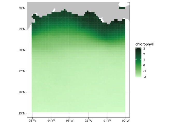
Get monthly MODIS data, which starts in 2002.
dataInfo <- rerddap::info('erdMH1chlamday_R2022SQ', url=ERDDAP_Node)
# Extract the parameter name from the metadata in dataInfo
parameter <- dataInfo$variable$variable_name

#Extract the start and end times of the dataset from the metadata in dataInfo
global <- dataInfo$alldata$NC_GLOBAL

# Populate the time vector with the time_coverage_start from dataInfo
# Use the "last" option for the ending date
tt <- global[ global$attribute_name %in% c('time_coverage_end','time_coverage_start'), "value", ]
tcoord <- c(tt[2],"last")

#Run rxtracto_3D
chlMODIS<-rxtracto_3D(dataInfo,
                      parameter=parameter,
                      tcoord=tcoord,
                      xcoord=xcoord,
                      ycoord=ycoord)
Get monthly VIIRS data, which starts in 2012.
dataInfo <- rerddap::info('nesdisVHNSQchlaMonthly', url=ERDDAP_Node)
# Extract the parameter name from the metadata in dataInfo
parameter <- dataInfo$variable$variable_name

#Extract the start and end times of the dataset from the metadata in dataInfo
global <- dataInfo$alldata$NC_GLOBAL

# This dataset has an altitude dimensionm, so must include zcoord as an argument in the rxtracto_3D function Set the altitude coordinate to zero
zcoord <- 0.

# Populate the time vector with the time_coverage_start from dataInfo
# Use the "last" option for the ending date
tt <- global[ global$attribute_name %in% c('time_coverage_end','time_coverage_start'), "value", ]
tcoord <- c(tt[2],"last")

#Run rxtracto_3D
chlVIIRS <- rxtracto_3D(dataInfo,
                      parameter=parameter,
                      tcoord=tcoord,
                      xcoord=xcoord,
                      ycoord=ycoord,
                      zcoord=zcoord)

# Remove extraneous zcoord dimension for chlorophyll
chlVIIRS$chlor_a <- drop(chlVIIRS$chlor_a)
Average data spatially and temporally
- spatially averages data for each time step within the area boundaries for each dataset.
- temporally averages data for data in each timeseries onto a map, for each dataset.
## Spatially average all the data within the box for each dataset.
## The c(3) indicates the dimension to keep - in this case time
chlSeaWiFS$avg <- apply(chlSeaWiFS$chlorophyll, c(3),function(x) mean(x,na.rm=TRUE))
chlMODIS$avg <- apply(chlMODIS$chlor_a, c(3),function(x) mean(x,na.rm=TRUE))
chlVIIRS$avg <- apply(chlVIIRS$chlor_a, c(3),function(x) mean(x,na.rm=TRUE))

## Temporally average all of the data into one map
## The c(1,2) indicates the dimensions to keep - in this case latitude and longitude
chlSeaWiFS$avgmap <- apply(chlSeaWiFS$chlorophyll,c(1,2),function(x) mean(x,na.rm=TRUE))
chlMODIS$avgmap <- apply(chlMODIS$chlor_a,c(1,2),function(x) mean(x,na.rm=TRUE))
chlVIIRS$avgmap <- apply(chlVIIRS$chlor_a,c(1,2),function(x) mean(x,na.rm=TRUE))
Plot time series for the three datasets
plot(as.Date(chlSeaWiFS$time), chlSeaWiFS$avg, type='l', col=2,lwd=2,
     xlab="", xlim=as.Date(c("1997-12-01","2024-06-01")),
     ylim=c(0.5,3.5), ylab="CHL")
axis(2)
points(as.Date(chlSeaWiFS$time), chlSeaWiFS$avg,pch=20,col=2)

lines(as.Date(chlMODIS$time), chlMODIS$avg, col=4, lwd=2)
points(as.Date(chlMODIS$time), chlMODIS$avg,pch=20,col=4)

lines(as.Date(chlVIIRS$time), chlVIIRS$avg, col=3, lwd=2)
points(as.Date(chlVIIRS$time), chlVIIRS$avg,pch=20,col=3)

legend('topleft',legend=c('SeaWiFS','MODIS','VIIRS'),cex=0.6,col=c(2,4,3),lwd=2)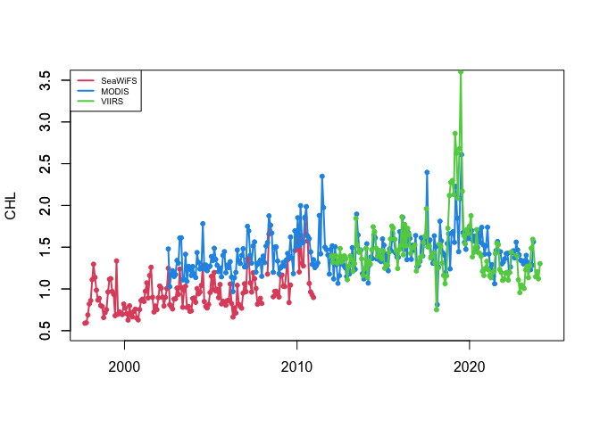
You can see that the values of chl-a concentration doesn’t always match between sensors.
Get OC-CCI data (September 1997 to Dec 2022)
If you needed a single time series from 1997 to present, you would have to use the plot above to devise some method to reconcile the difference in values where two datasets overlap. Alternatively, you could use the ESA OC-CCI (ocean color climate change initiative) dataset, which blends data from many satellite missions into a single dataset, including data from SeaWiFS, MODIS, and VIIRS.
Add the ESA OC-CCI dataset to the plot above to see how it compares with data from the individual satellite missions.
dataInfo <- rerddap::info('pmlEsaCCI60OceanColorMonthly', url=ERDDAP_Node)

# This identifies the parameter to choose - there are > 60 in this dataset!
parameter <- 'chlor_a'

global <- dataInfo$alldata$NC_GLOBAL
tt <- global[ global$attribute_name %in% c('time_coverage_end','time_coverage_start'), "value", ]
tcoord <- c(tt[2],"last")

chlOCCCI<-rxtracto_3D(dataInfo,
                      parameter=parameter,
                      tcoord=tcoord,
                      xcoord=xcoord,
                      ycoord=ycoord)

# Now spatially average the data into a timeseries
chlOCCCI$avg <- apply(chlOCCCI$chlor_a, c(3),function(x) mean(x,na.rm=TRUE))

# Now temporally average the data into one map
chlOCCCI$avgmap <- apply(chlOCCCI$chlor_a,c(1,2),function(x) mean(x,na.rm=TRUE))
Make another plot with CCI as well to compare
plot(as.Date(chlSeaWiFS$time), chlSeaWiFS$avg, type='l', col=2,lwd=2,
     xlab="", xlim=as.Date(c("1997-12-01","2024-06-01")),
     ylim=c(0.5,3.5), ylab="CHL")
axis(2)
points(as.Date(chlSeaWiFS$time), chlSeaWiFS$avg,pch=20,col=2)
points(as.Date(chlMODIS$time), chlMODIS$avg,pch=20,col=4)
points(as.Date(chlVIIRS$time), chlVIIRS$avg,pch=20,col=3)
lines(as.Date(chlOCCCI$time),chlOCCCI$avg,lwd=2)

legend('topleft',legend=c('SeaWiFS','MODIS','VIIRS','OC-CCI'),cex=0.6,col=c(2,4,3,1),
       pch=c(20,20,20,NA),lty=c(NA,NA,NA,1),lwd=2)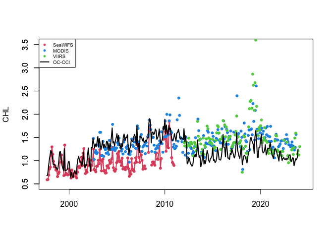
coast <- map_data("worldHires", ylim = ycoord, xlim = xcoord)
# Put arrays into format for ggplot
melt_map <- function(lon,lat,var) {
dimnames(var) <- list(Longitude=lon, Latitude=lat)
ret <- melt(var,value.name="Chl")
}
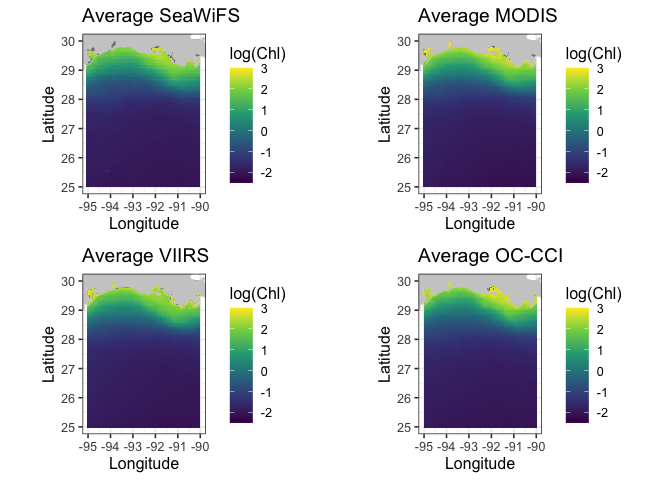
# Loop for making 4 maps
datasetnames <- c("SeaWiFS","MODIS","VIIRS","OC-CCI")
plot_list = list()
for(i in 1:4) {
if(i == 1) chl <- chlSeaWiFS
if(i == 2) chl <- chlMODIS
if(i == 3) chl <- chlVIIRS
if(i == 4) chl <- chlOCCCI
chlmap <- melt_map(chl$longitude, chl$latitude, chl$avgmap)
p = ggplot(
data = chlmap,
aes(x = Longitude, y = Latitude, fill = log(Chl))) +
geom_tile(na.rm=T) +
geom_polygon(data = coast, aes(x=long, y = lat, group = group), fill = "grey80") +
theme_bw(base_size = 12) + ylab("Latitude") + xlab("Longitude") +
coord_fixed(1.3, xlim = c(-95,-90), ylim = ycoord) +
scale_fill_viridis_c(limits=c(-2.5,3)) +
ggtitle(paste("Average", datasetnames[i])
)
plot_list[[i]] = p
}
# Now print out maps into a png file. Can't use par function with **ggplpot** to get
# multiple plots per page. Here using a function in the **grid** package
grid.arrange(plot_list[[1]],plot_list[[2]],plot_list[[3]],plot_list[[4]], nrow = 2)