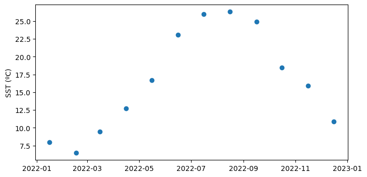
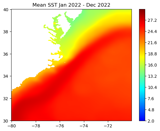
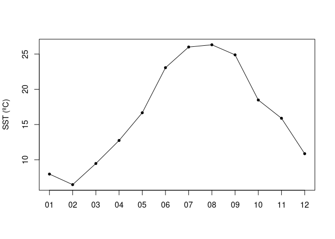
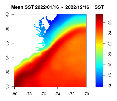
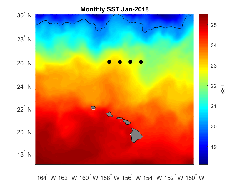
Basics of working with satellite data
Access and analyze satellite-derived sea surface temperature using ERDDAP and NetCDF-based workflows. This tutorial demonstrates how to locate and subset a satellite SST product in ERDDAP, download gridded NetCDF data, examine its structure, and create basic spatial maps and regional time series. Users work with the NOAA Coral Reef Watch CoralTemp monthly sea surface temperature product to explore coordinate conventions, generate SST maps, compute regional averages, and visualize temporal variability.
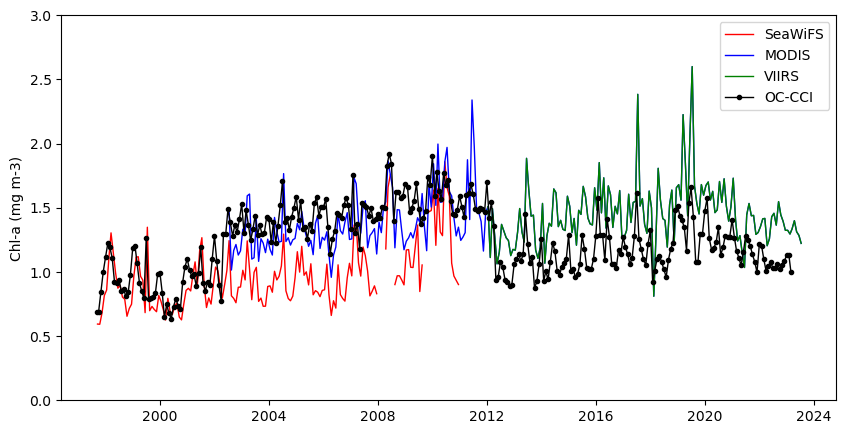
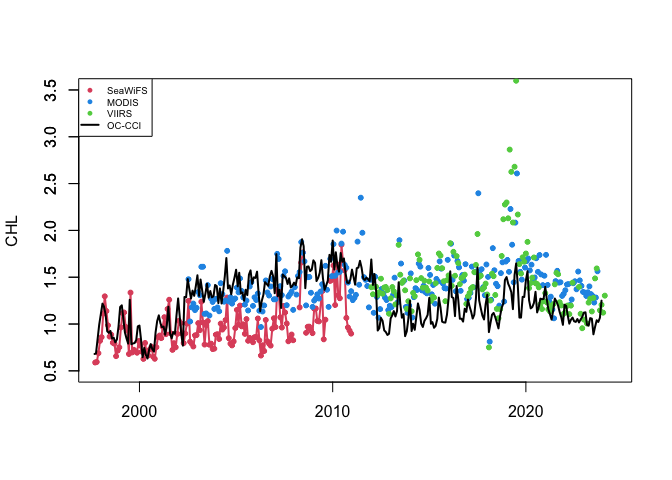
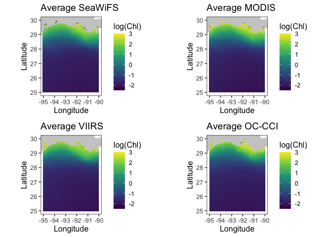
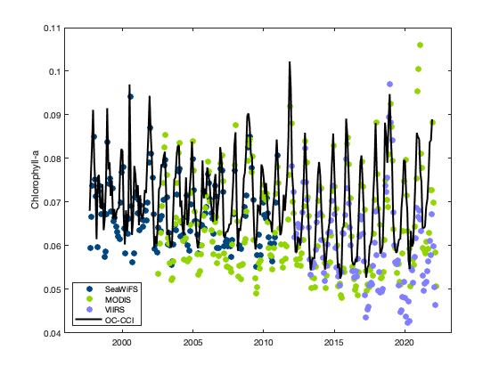
Compare time series from different sensors
Compare satellite chlorophyll-a time series from multiple ocean color sensors to understand differences during overlapping observation periods. This tutorial demonstrates how to use ERDDAP to extract spatially averaged chlorophyll-a time series from a defined region, examine dataset metadata, handle differences in coordinate conventions, and compare measurements across sensors through visualization. Monthly chlorophyll-a data from SeaWiFS, MODIS Aqua, NOAA VIIRS S-NPP, and the ESA Ocean Colour Climate Change Initiative (OC-CCI) are used to evaluate consistency and variability among sensors from 1997 to the present.
Make a virtual buoy with satellite data
Create a virtual ocean buoy using satellite data to extend or replace discontinued in situ observations. This tutorial demonstrates how to use ERDDAP to extract satellite sea surface temperature at a fixed location, build and clean a virtual buoy time series, resample the data to a lower temporal resolution, and analyze trends through visualization and linear regression. Data from NDBC Buoy 46259 are used alongside the NOAA GeoPolar Blended SST satellite dataset.
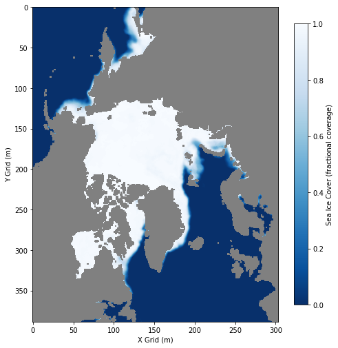
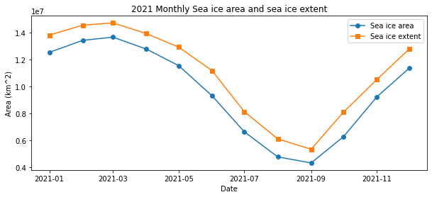
Calculating sea ice area and extent
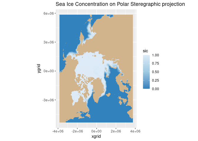
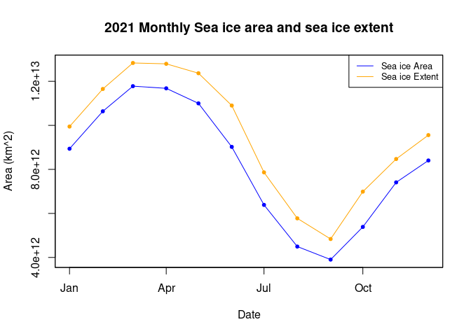
Calculate sea ice area and extent from satellite-derived sea ice concentration to quantify seasonal and interannual variability in Arctic ice cover. This tutorial demonstrates how to use PolarWatch ERDDAP to retrieve gridded sea ice concentration data, incorporate grid cell area information, and apply standard concentration thresholds to compute sea ice area and extent. Users visualize sea ice concentration maps and generate monthly time series to examine changes in Arctic sea ice over time. Data from the NOAA/NSIDC Sea Ice Concentration Climate Data Record (Version 4) and a polar stereographic grid cell area dataset are used to perform the calculations for the Northern Hemisphere.
Working with data that crosses the antimeridian
Work with satellite datasets that span the antimeridian by correcting longitude discontinuities for analysis and visualization. This tutorial demonstrates how to retrieve gridded satellite data defined on a −180° to +180° longitude system, subset regions that cross the antimeridian, convert longitude coordinates to a 0–360° system, and reorder the longitude axis to create a continuous spatial domain. The corrected data are then visualized on a map and saved for downstream analysis. Chlorophyll-a data from the NOAA gap-filled blended VIIRS ocean color dataset are used to illustrate antimeridian handling in the Bering Sea region.
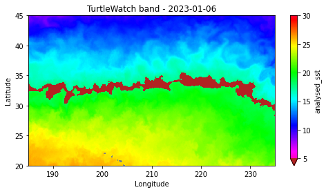
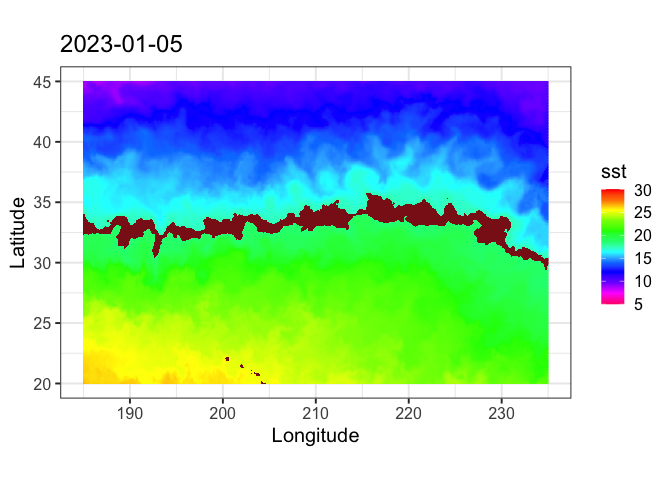
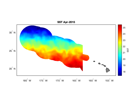
Define a marine habitat
Define a marine habitat using satellite sea surface temperature to identify regions associated with species–environment interactions. This tutorial demonstrates how to retrieve satellite SST from ERDDAP, subset data for a region and time of interest, and apply temperature-based thresholds to delineate a habitat band. The resulting temperature contours are visualized on a map to highlight areas associated with increased likelihood of interaction. Sea surface temperature data from the NOAA Coral Reef Watch CoralTemp product are used to illustrate habitat definition in the central North Pacific as part of the TurtleWatch framework.
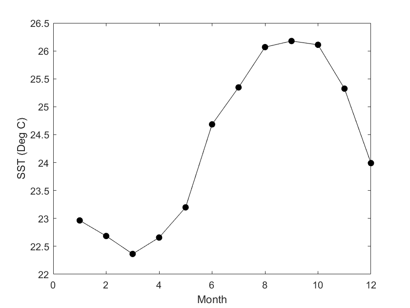
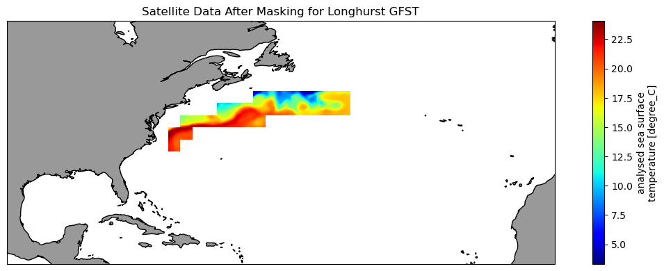
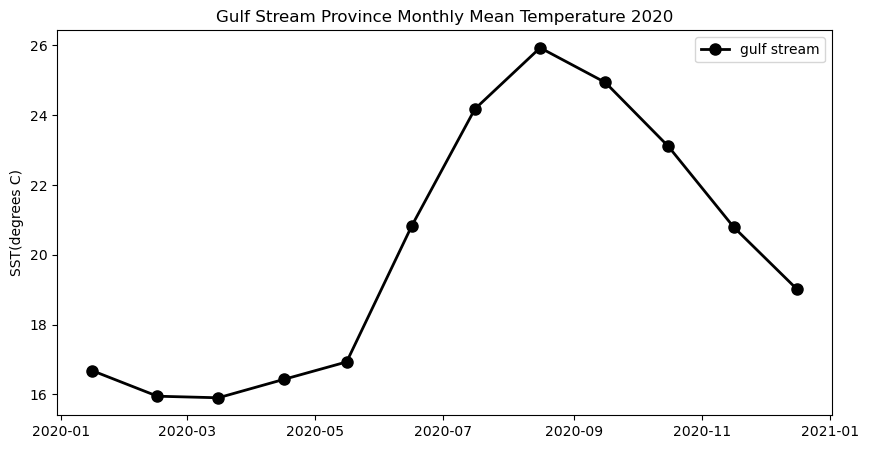
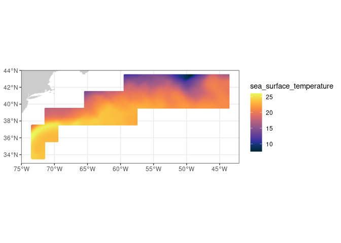
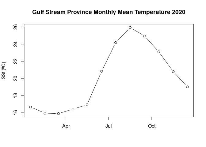
Extract data within a boundary
Extract and analyze satellite data within an irregular geographic boundary to better represent real-world marine regions. This tutorial demonstrates how to download sea surface temperature data from ERDDAP, subset it using a bounding box, and apply a polygon mask to retain values only within a defined boundary. The masked data are then used to compute and visualize a seasonal temperature cycle for the region of interest. Sea surface temperature data from the NOAA Geo-Polar Blended SST product are combined with Longhurst Marine Province boundaries to illustrate region-based satellite analysis.
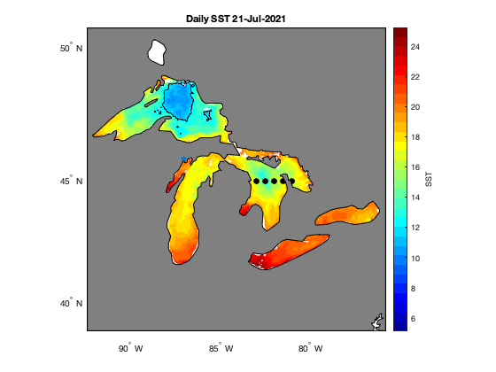
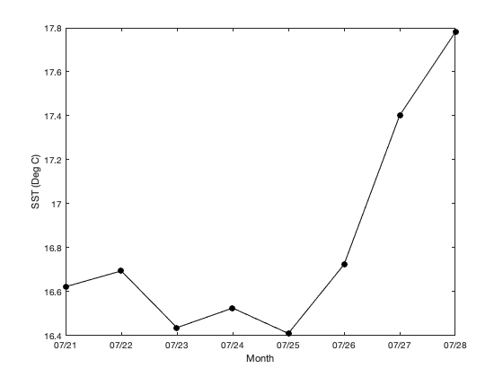
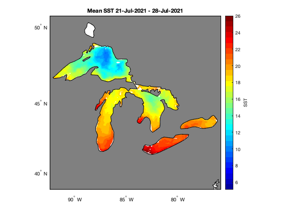
How to work with satellite data in Matlab in the Great Lakes
Access and analyze satellite sea surface temperature data in MATLAB using ERDDAP and NetCDF workflows. This tutorial demonstrates how to construct ERDDAP download URLs, read NetCDF variables directly into MATLAB, convert time coordinates, and subset data spatially and temporally. The workflow includes creating daily SST maps, generating regional mean time series, and computing average SST over a selected period. Satellite sea surface temperature data from NOAA CoastWatch are used to illustrate spatial and temporal analysis across the Great Lakes region.
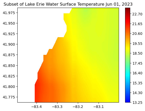
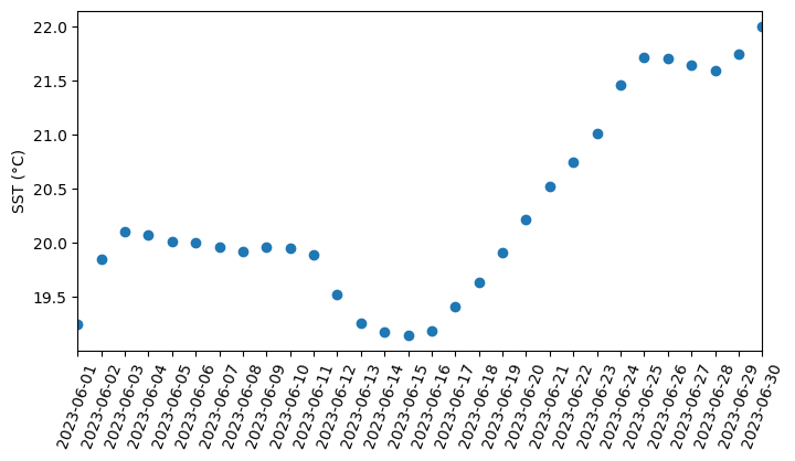
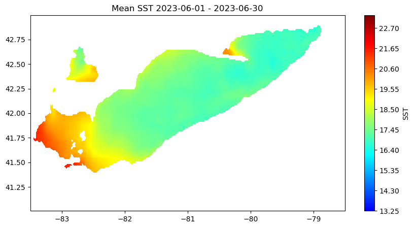
Working with Great Lakes Surface Temperature Data
Access and analyze Great Lakes surface temperature using satellite observations in Python. This tutorial demonstrates how to download water surface temperature data from an ERDDAP server, open and inspect NetCDF files using xarray, and convert time variables into usable date formats. The extracted data are used to generate spatial maps of surface temperature, compute regional averages within user-defined bounding boxes, and visualize temporal variability through daily time series and monthly mean maps. Water surface temperature data from the Great Lakes Surface Environmental Analysis (GLSEA) ACSPO dataset are used to illustrate satellite-based analysis of Lake Erie.
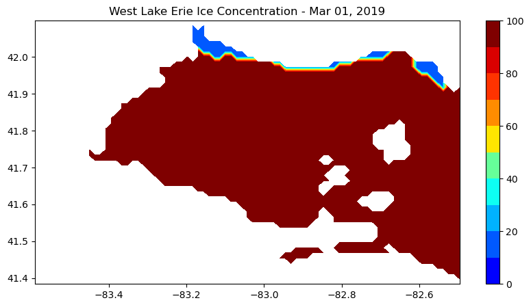
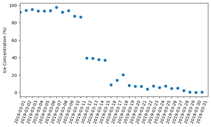
Analyze Great Lakes Ice Concentration
Extract and summarize satellite-derived ice concentration to characterize seasonal ice conditions in the Great Lakes. This tutorial demonstrates how to download ice concentration data from ERDDAP, subset the data spatially and temporally for a region of interest, and handle missing values in NetCDF files. The extracted data are used to generate maps of ice concentration for specific dates and to compute regional daily mean ice concentration time series. Ice concentration data from the NOAA Great Lakes Surface Environmental Analysis (GLSEA) product are used to illustrate regional ice variability in western Lake Erie.
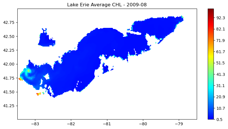
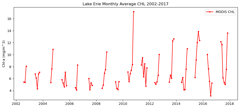
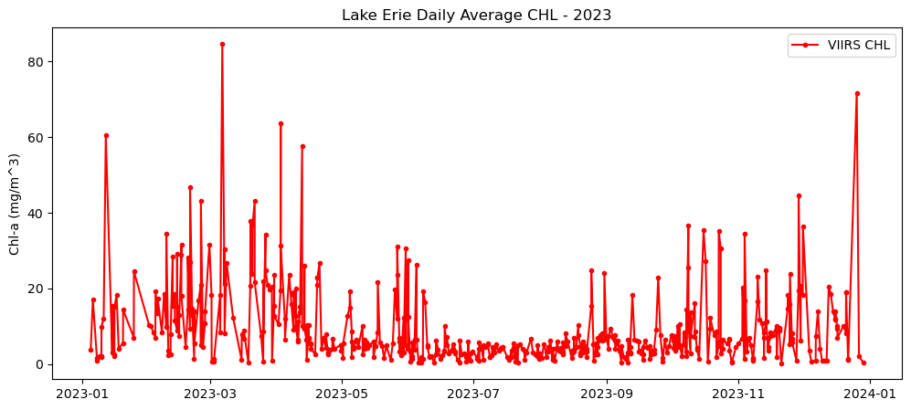
Multi-Sensor chlorophyll time series analysis for Lake Erie
Analyze long-term changes in lake chlorophyll concentrations by combining satellite observations from multiple sensors. This tutorial demonstrates how to download chlorophyll-a data from ERDDAP for Lake Erie, process daily observations from MODIS (2002–2017) and VIIRS (2018–2023), and compute spatially averaged monthly and daily time series. The workflow shows how to handle fill values, aggregate data across space and time, and visualize chlorophyll variability across the sensor transition. By merging MODIS and VIIRS records, the tutorial provides a practical approach for creating a continuous multi-sensor time series to support long-term water quality analysis in the Great Lakes.
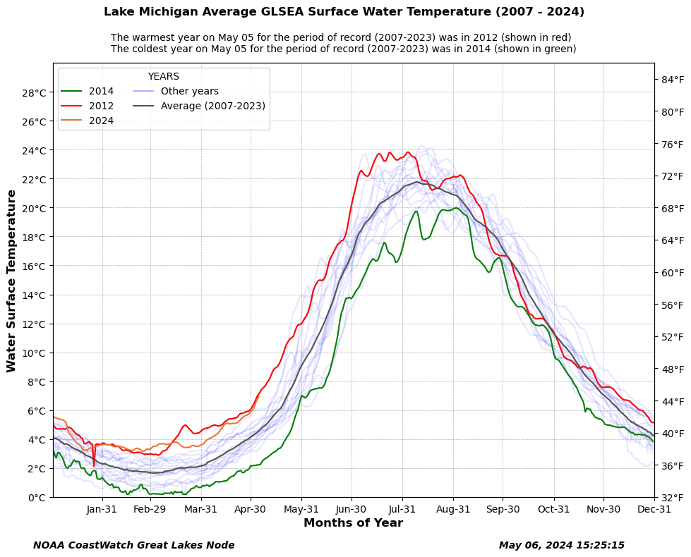
Long-term lake surface temperature variability from Great Lakes Satellite Records
Analyze long-term patterns in Great Lakes water surface temperature using lakewide satellite-derived averages. This tutorial demonstrates how to retrieve daily average surface temperature data from ERDDAP, assemble a multi-year record spanning 2007 to the present, and visualize seasonal temperature variability across years. Daily temperature records are aligned by day of year to highlight the warmest, coldest, and average conditions for a given date, with the current year shown in context of the historical record. Using Great Lakes Surface Environmental Analysis (GLSEA) satellite products, the workflow illustrates how long-term lake temperature climatologies can be used to assess seasonal extremes and interannual variability across the Great Lakes.
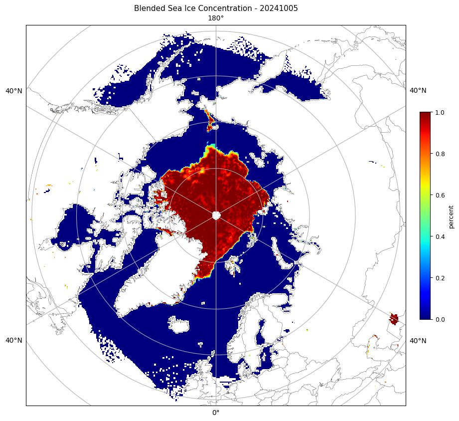
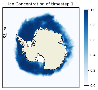
Visualizing JPSS Sea Ice Concentration products using Google Colab
Visualize polar sea ice conditions by converting JPSS Sea Ice Concentration files into mapped images for quick inspection and reporting. This tutorial demonstrates how to obtain either Level-2 swath VIIRS ice concentration data or Level-3 daily gridded blended sea ice concentration products, load them into an analysis environment, and generate publication-ready maps for the Arctic or Antarctic. The workflow resamples swath observations onto a common polar grid when needed, applies consistent color scaling in percent ice concentration, and exports the final figures as PNGs.
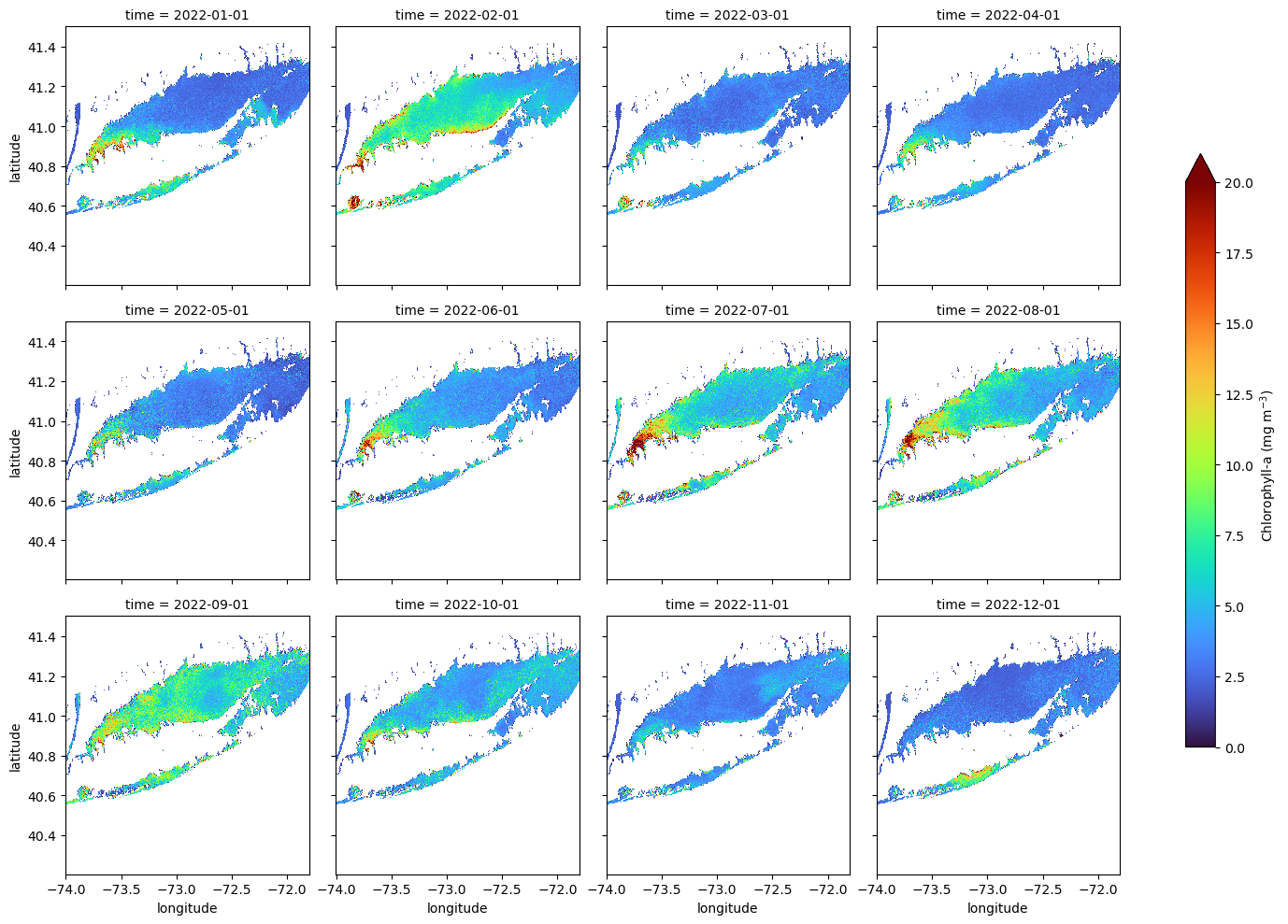
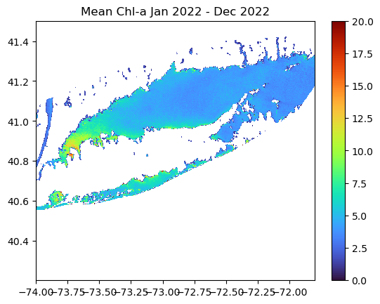
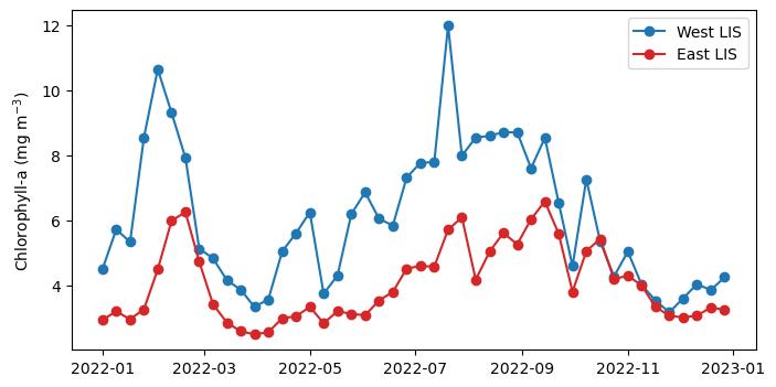
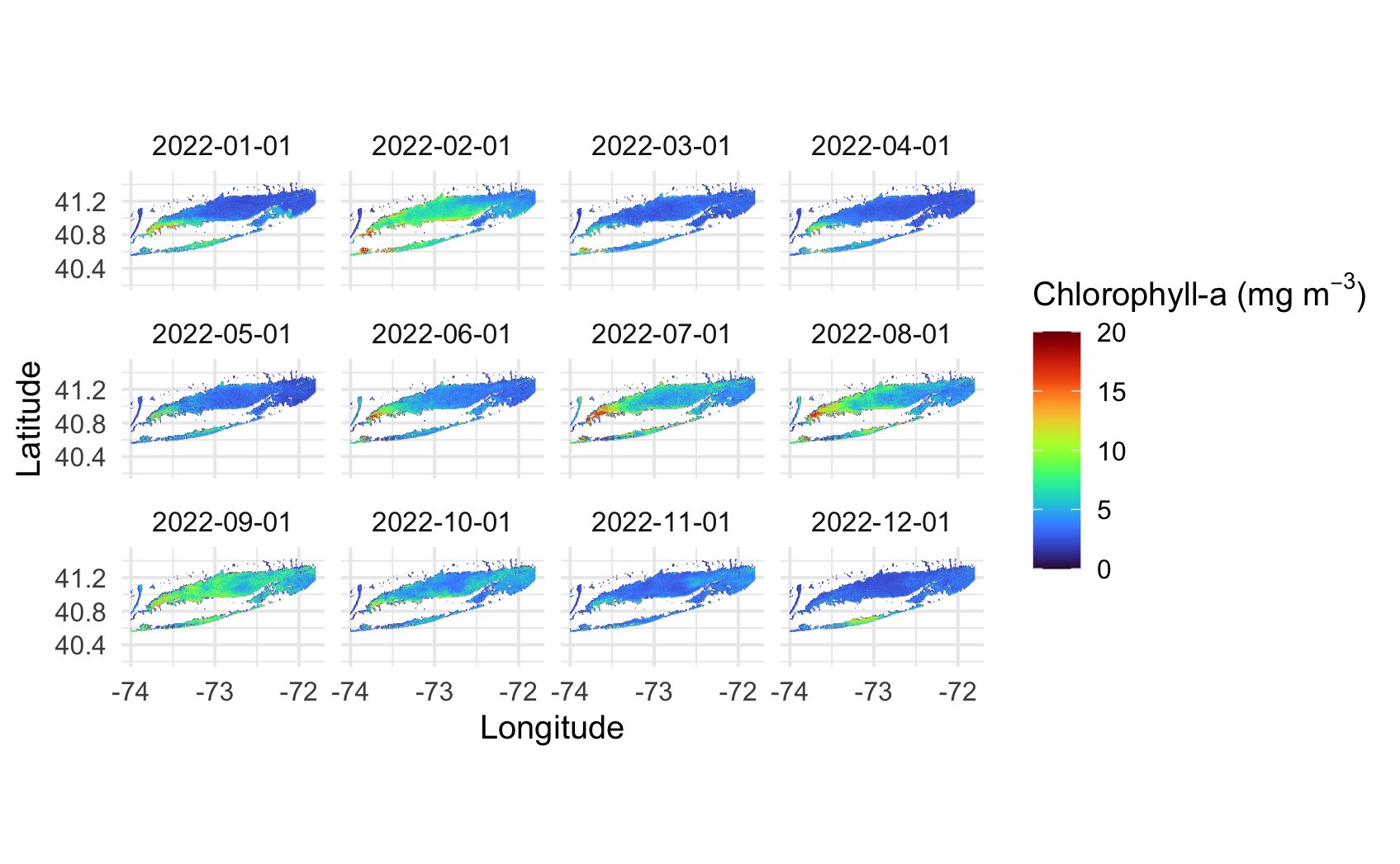
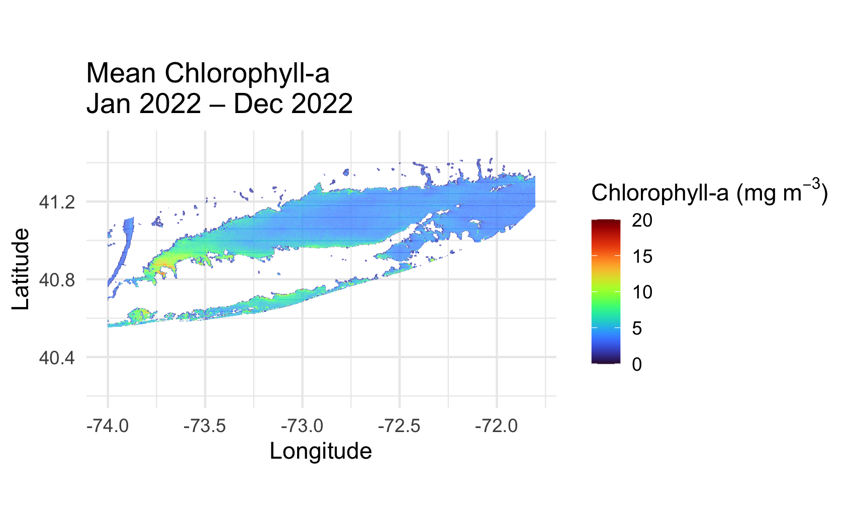
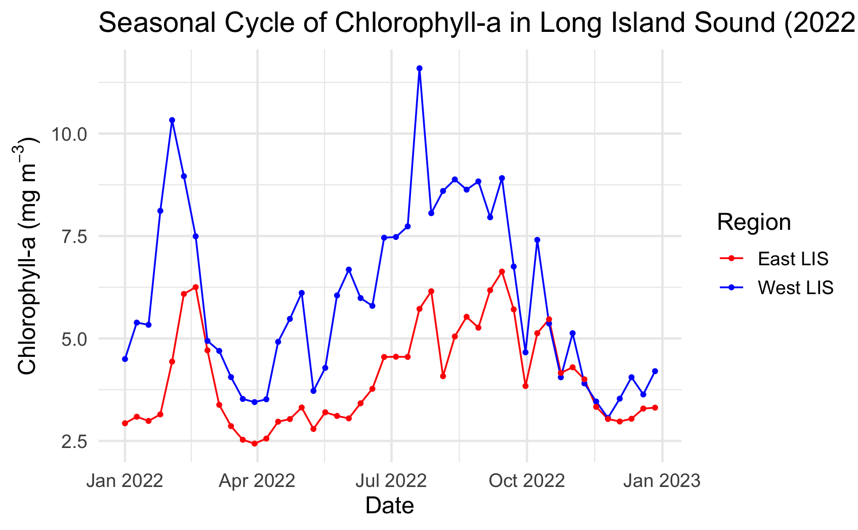
Long Island Sound Chlorophyll-a Dynamics
Analyze seasonal and spatial patterns in coastal chlorophyll-a by working with daily satellite observations from Long Island Sound. This tutorial demonstrates how to download chlorophyll-a data from ERDDAP, generate temporal composites at monthly and 8-day intervals, and subset the data to compare regional variability within the Sound. The workflow illustrates how to examine gridded satellite datasets, compute spatial averages, and visualize chlorophyll dynamics through maps and time-series plots. Chlorophyll-a data from Sentinel-3 OLCI, processed with Long Island Sound–optimized algorithms, are used to highlight differences between western and eastern regions and to explore seasonal water-quality variability in a complex coastal environment.
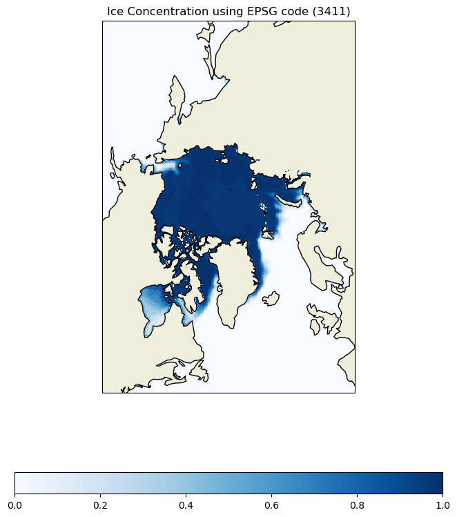
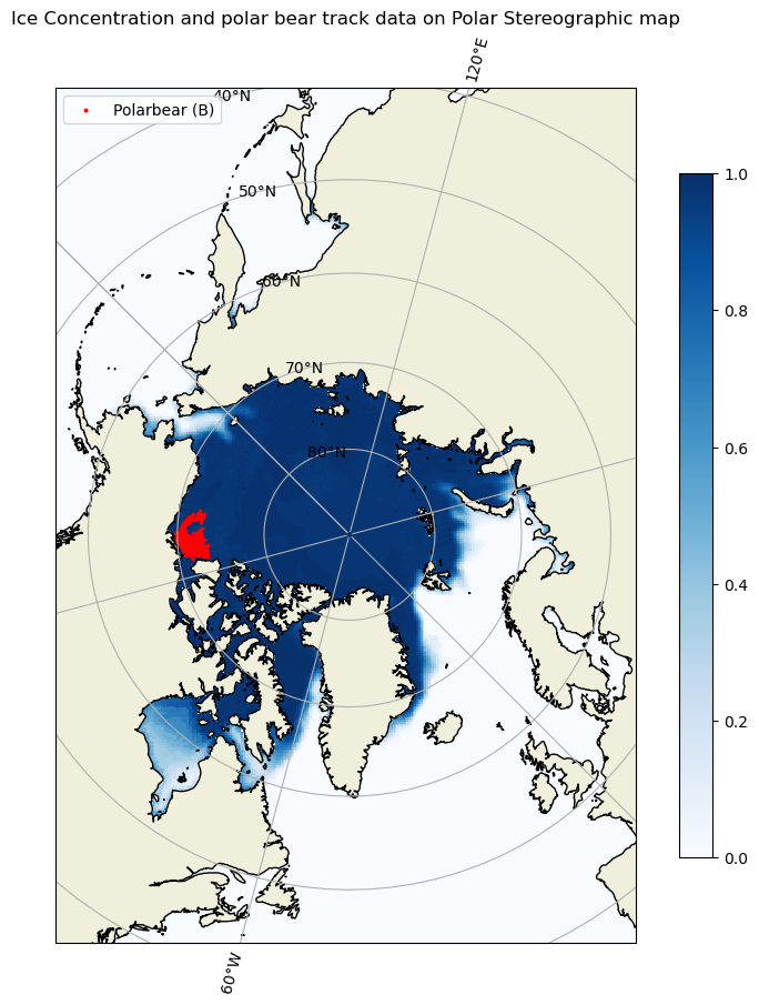
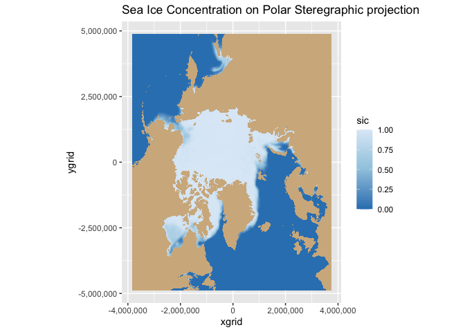
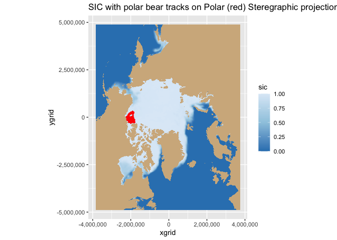
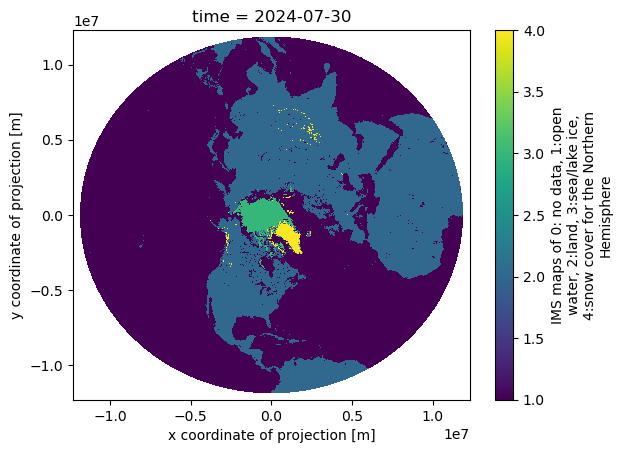
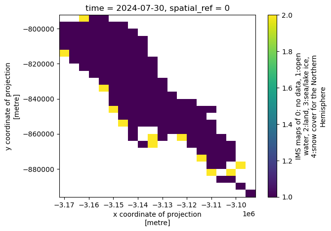
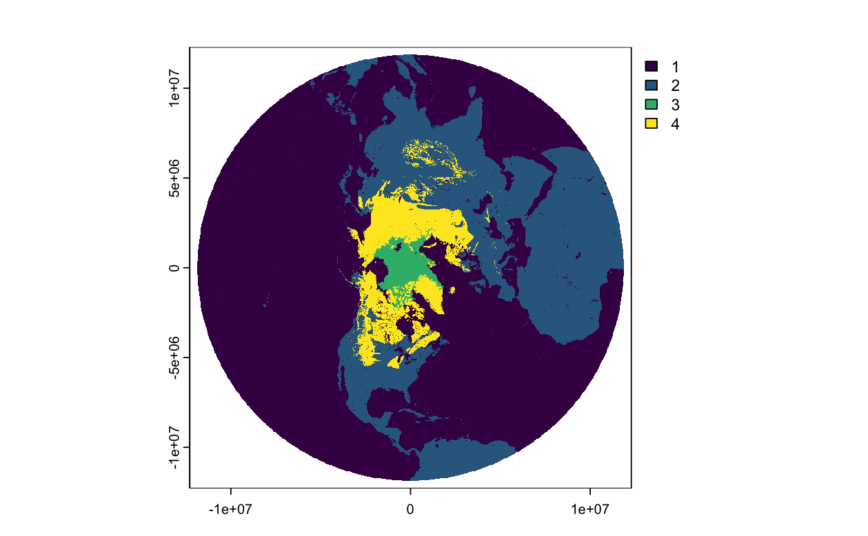
Map geographical and polarstereographic data on a projected map
Plot polar satellite data correctly by working across coordinate systems and projections. This tutorial demonstrates how to access polar sea ice concentration data from an ERDDAP server, interpret the dataset’s polar stereographic metadata (or EPSG code), and display the gridded x–y product on a matching projected basemap. It then shows how to overlay a second dataset provided in geographic coordinates (latitude/longitude) here, polar bear GPS tracks by transforming those points into the same map projection for direct visual comparison with the sea ice field.
Mask shallow pixels for satellite ocean color datasets
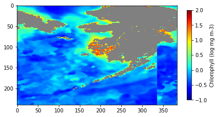
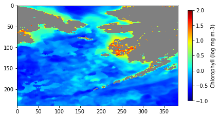
Remove optically shallow-water contamination from satellite ocean color data to improve the accuracy of derived biogeochemical metrics. This tutorial demonstrates how to download bathymetry and monthly chlorophyll-a data from ERDDAP, quantify the fraction of shallow water within each ocean color pixel, and construct a threshold-based mask to exclude pixels affected by bottom reflectance. The masked and unmasked datasets are then used to compute and compare long-term chlorophyll-a climatologies. By combining high-resolution bathymetry with coarse-resolution ocean color observations, the workflow illustrates a practical approach for preparing satellite datasets for robust analysis in coastal and reef-adjacent regions.
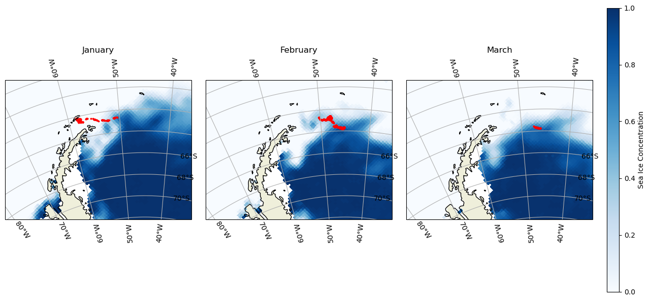
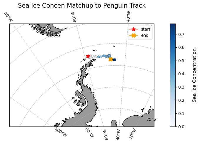
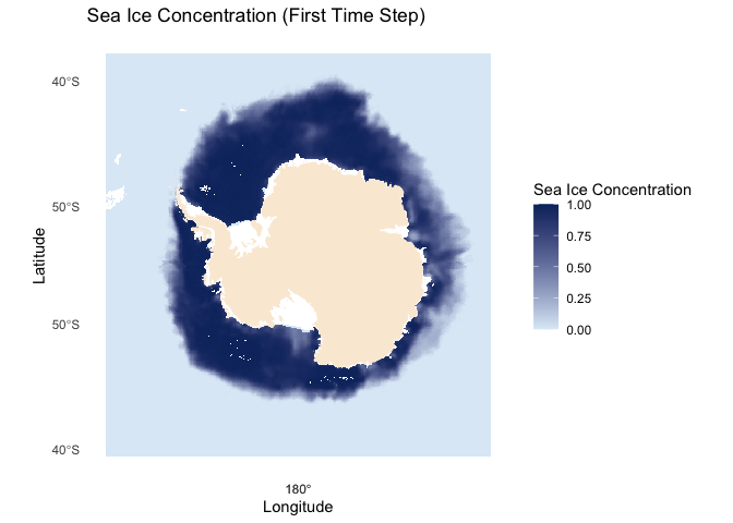
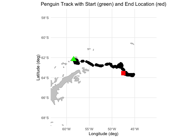
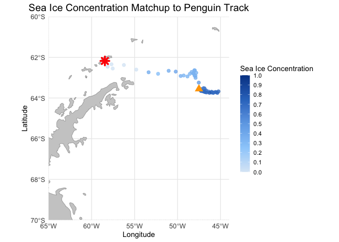
Matching polar data to animal track locations
Extract and analyze satellite sea ice conditions along animal movement tracks in polar regions. This tutorial demonstrates how to combine satellite sea ice concentration data with animal telemetry observations to examine environmental conditions encountered along a tracked path. Using monthly sea ice concentration records from NOAA PolarWatch, the workflow shows how to subset gridded satellite data in polar stereographic coordinates, align it temporally and spatially with penguin telemetry locations, and extract coincident sea ice values along the track. The tutorial also illustrates how to visualize animal movement overlaid on sea ice maps and how to generate matched time series of satellite-derived sea ice concentration at each observation point.
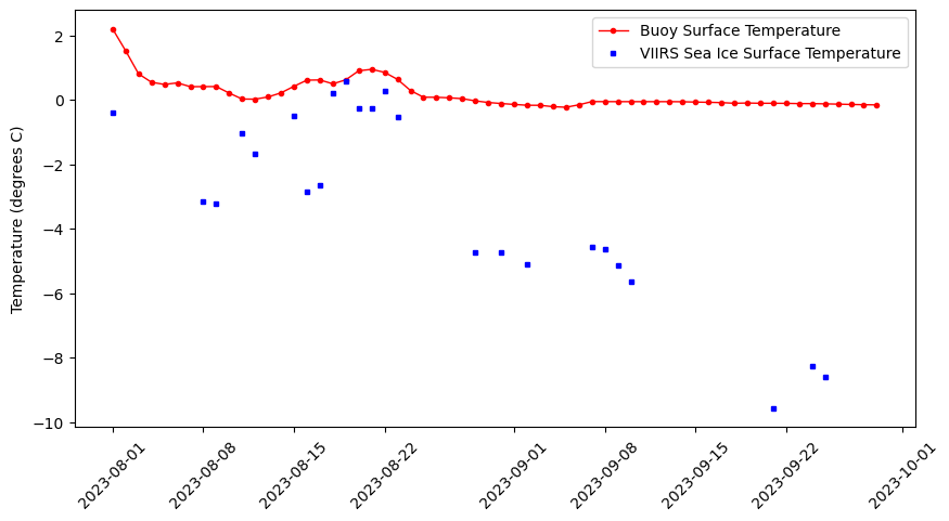
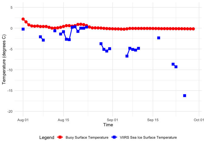
Matching satellite and buoy surface temperature data in polar regions
Combine satellite ice surface temperature composites with in situ buoy observations by matching satellite pixels to buoy locations and dates in the Arctic. This tutorial walks through how to query buoy surface temperature records from ERDDAP in tabular format, download polar-projected satellite Ice Surface Temperature (IST) data in NetCDF, and resample the buoy time series to comparable time steps. It then demonstrates how to convert buoy latitude/longitude positions into the satellite’s polar stereographic coordinate system, extract the nearest satellite IST values at each buoy time and location, and merge the two datasets for side-by-side comparison and visualization.
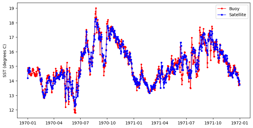
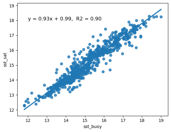
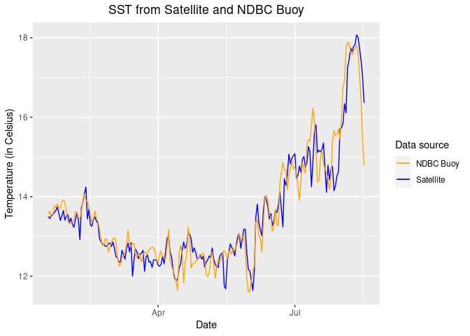
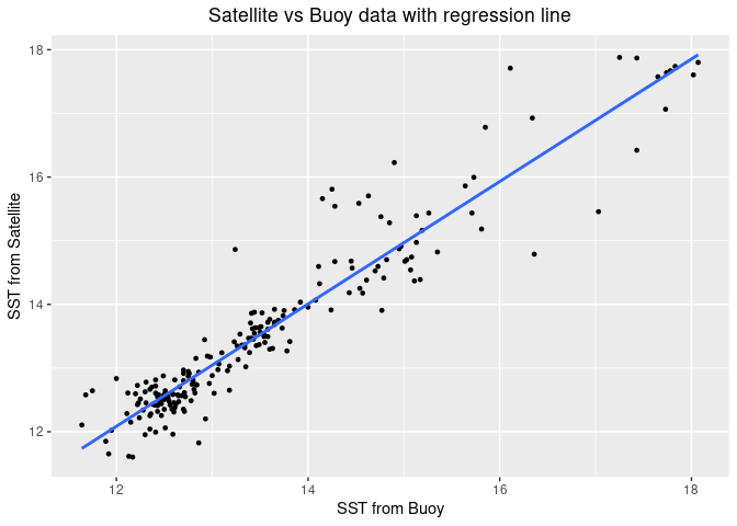
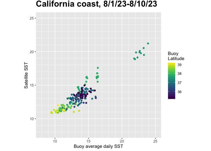
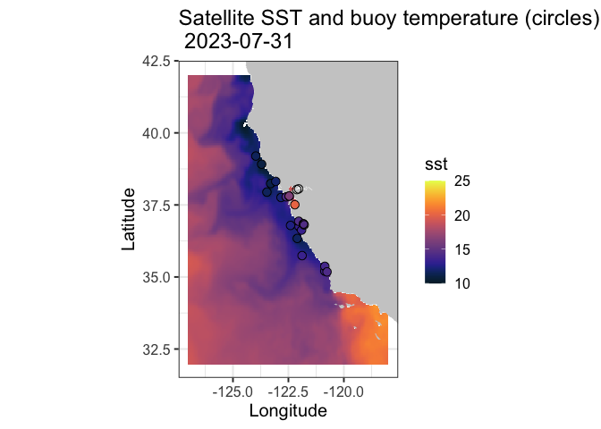
Comparing satellite and buoy sea surface temperature observations
This tutorial demonstrates how to match satellite-derived sea surface temperature (SST) with in situ buoy observations to evaluate satellite data accuracy. Using ERDDAP-hosted datasets, the workflow shows how to download and process buoy measurements, extract collocated satellite SST values, and compare the two datasets through statistical analysis and visualization.
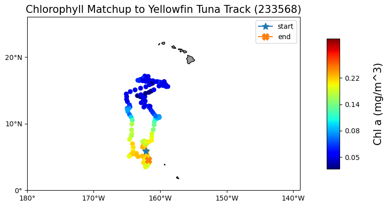
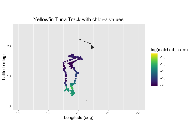
Matchup satellite data to ship, glider, or animal tracks
Extract and analyze satellite-derived environmental variables along moving platforms such as ship tracks, gliders, or animal telemetry paths. This tutorial demonstrates how to load track data defined by latitude, longitude, and time, visualize trajectories on a map, and retrieve colocated satellite observations from ERDDAP for each track position. Using a yellowfin tuna telemetry record as an example, satellite chlorophyll-a data from the ESA Ocean Colour Climate Change Initiative are matched to daily track locations, saved to a tabular format, and visualized to explore spatial and temporal variability along the track.
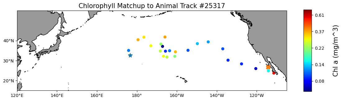
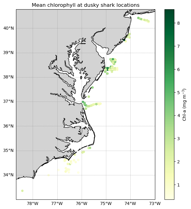
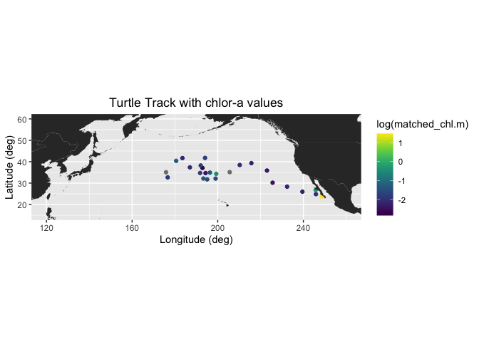
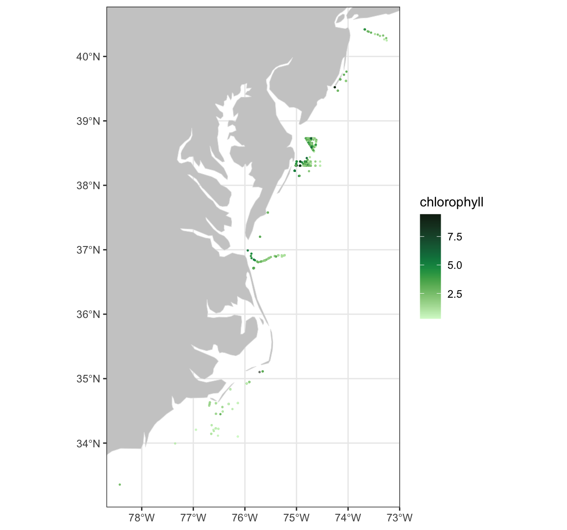
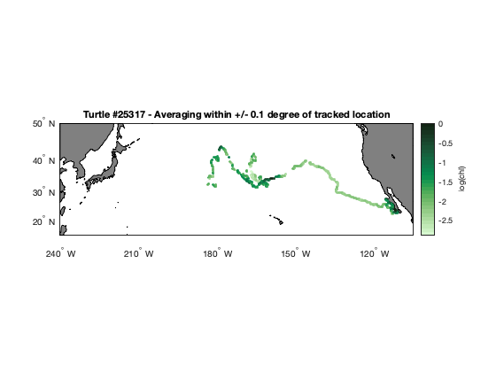
Matching satellite chlorophyll to animal telemetry tracks
This tutorial demonstrates how to match satellite chlorophyll data to animal, ship, or glider tracks using longitude, latitude, and time coordinates. Examples include a loggerhead turtle track using nearest-pixel matchups and a dusky shark telemetry dataset that applies spatial averaging within a local window to better represent environmental conditions along movement tracks.
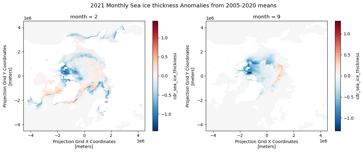
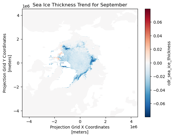
Calculating anomaly and trend with sea ice thickness time series
This tutorial demonstrates how to analyze variability and long-term change in Arctic sea ice thickness using gridded satellite data. Monthly mean sea ice thickness fields are derived from twice-daily observations accessed through the PolarWatch ERDDAP server, then compared against a multi-year climatological baseline to quantify anomalies. A 15-year reference period (2006–2020) is used to compute historical monthly means, which serve as the basis for anomaly calculations and trend assessment. Long-term trends in monthly sea ice thickness are estimated at each grid cell using the non-parametric Mann–Kendall method, allowing robust slope estimation without assumptions of normality.
Subset data in polar stereographic projection using a shapefile
This exercise demonstrates how to subset satellite data provided in a polar stereographic projection using a lake boundary defined in a different coordinate reference system. The workflow includes downloading polar satellite data from PolarWatch ERDDAP, transforming a shapefile to match the satellite projection, and clipping the dataset to the extent of Lake Iliamna in Alaska. The results are visualized to illustrate projection handling and spatial subsetting of polar remote sensing data
Transforming satellite data from one map to another
This exercise demonstrates how to transform satellite data coordinates from one map projection to another in order to work consistently with datasets that use different coordinate reference systems. It walks through downloading sea ice concentration data from PolarWatch ERDDAP, inspecting CRS definitions, applying EPSG-based coordinate transformations, and adding the transformed coordinates back into a NetCDF dataset.
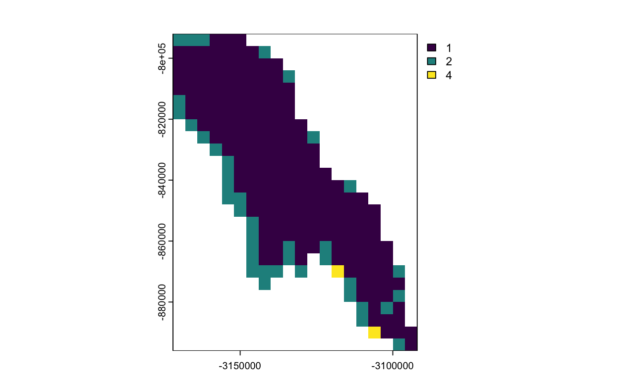
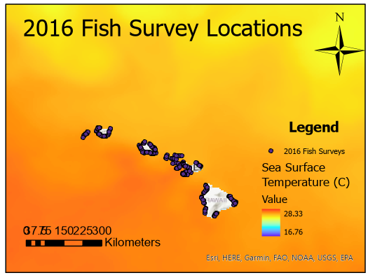
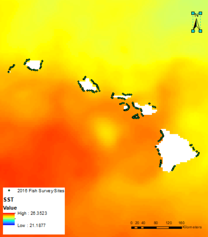
Working with Multidimensional SST Data in ArcGIS
This ArcGIS tutorial walks through a complete end-to-end SST workflow, from downloading NetCDF data from ERDDAP to importing and managing multidimensional raster data within ArcGIS. You will learn how to configure the time dimension, visualize monthly SST using the time slider, extract environmental values at survey locations and within polygons, calculate zonal statistics using the Spatial Analyst extension, and build a simple habitat suitability map based on an SST range. Parallel tutorials are available for both ArcGIS Pro and ArcMap, allowing you to follow the same workflow in the platform you use.

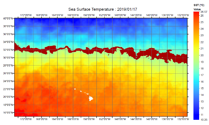
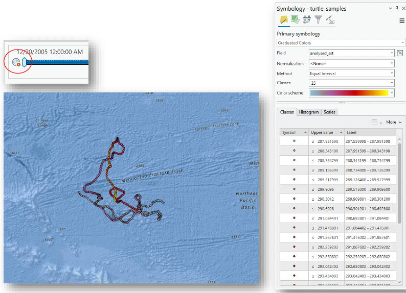
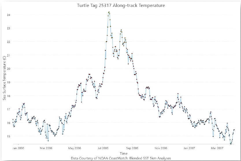
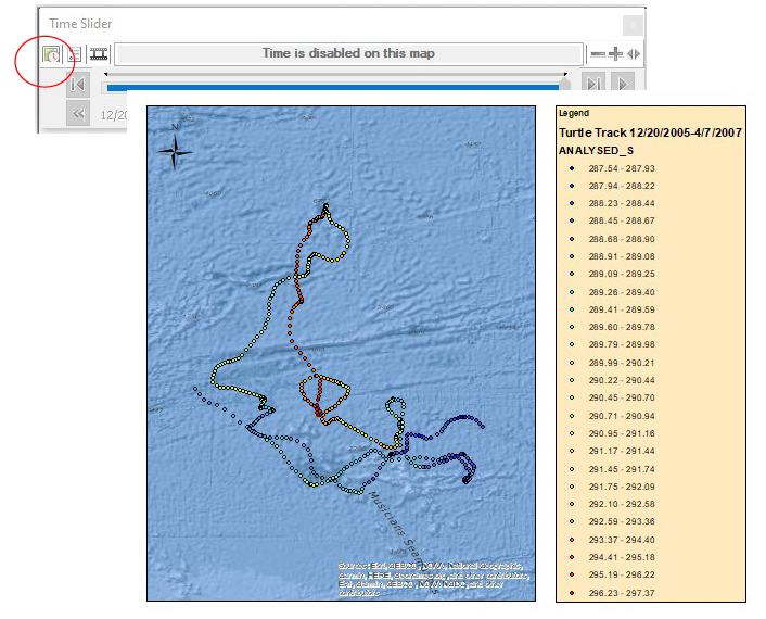
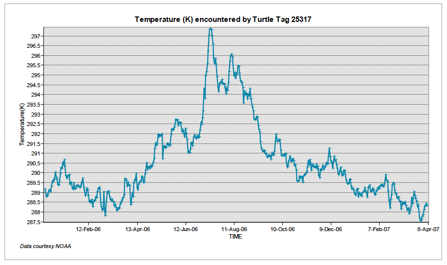
Using Satellite SST Data in ArcGIS
This tutorial demonstrates how to use Sea Surface Temperature (SST) data in ArcGIS to perform spatial and temporal analysis with multidimensional NetCDF datasets. Using a multi-year loggerhead sea turtle track example, you will import satellite data from ERDDAP, prepare and convert CSV tracking data, enable time-aware layers, extract raster values with the Spatial Analyst tools, and create maps, graphs, and animations. Parallel versions are provided for both ArcMap and ArcGIS Pro, following the same scientific workflow with platform-specific tools.
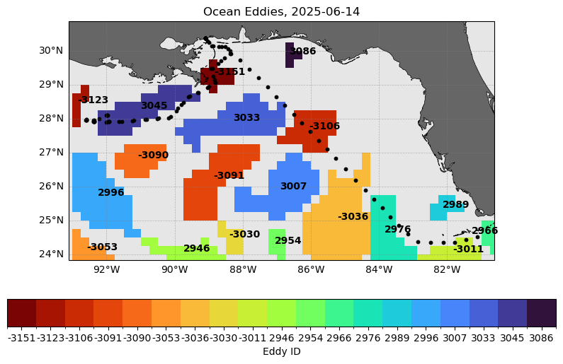
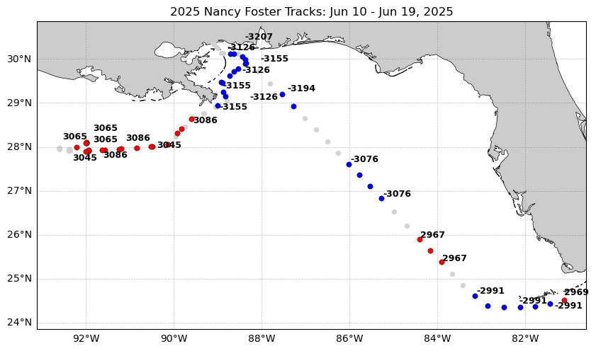
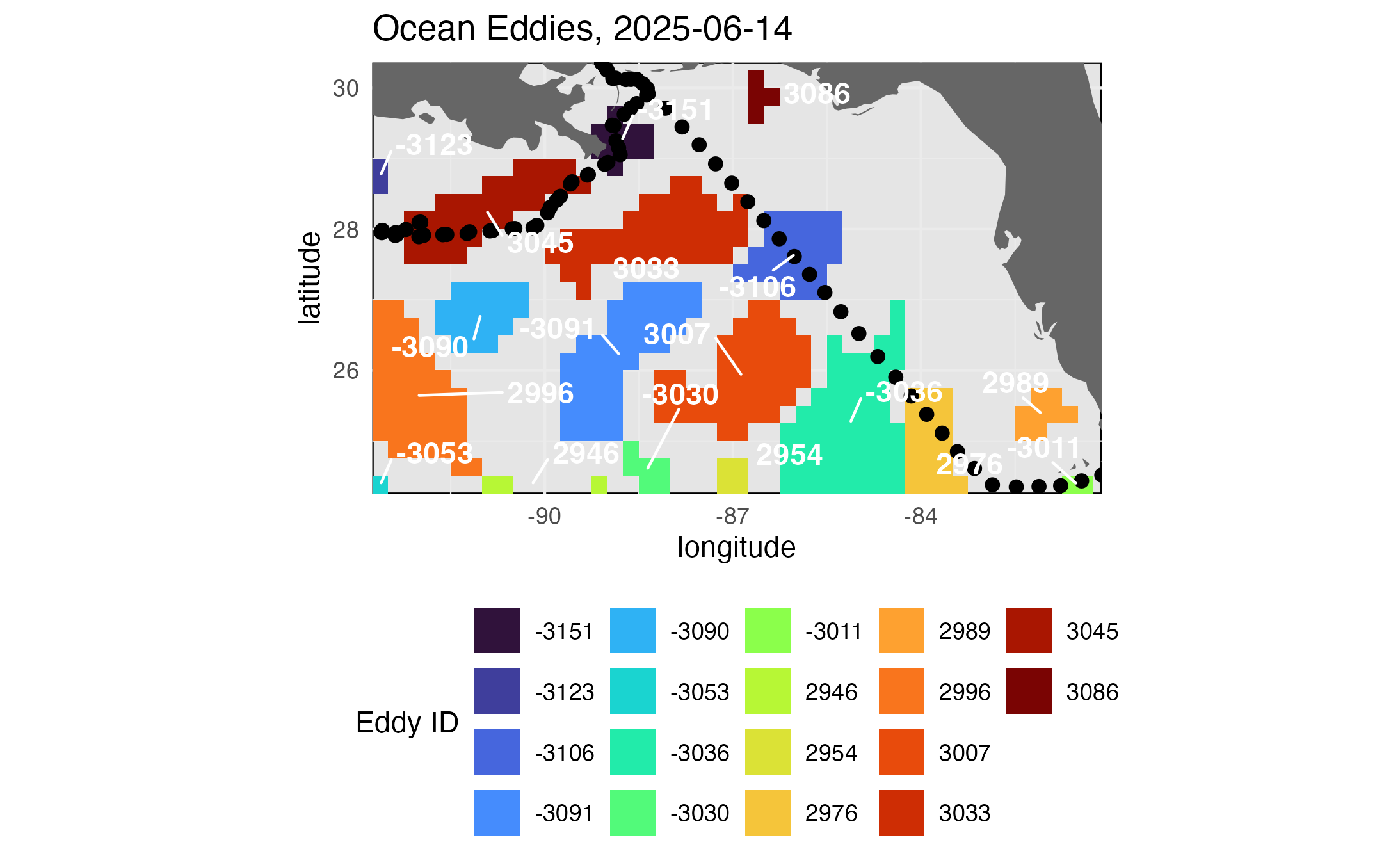
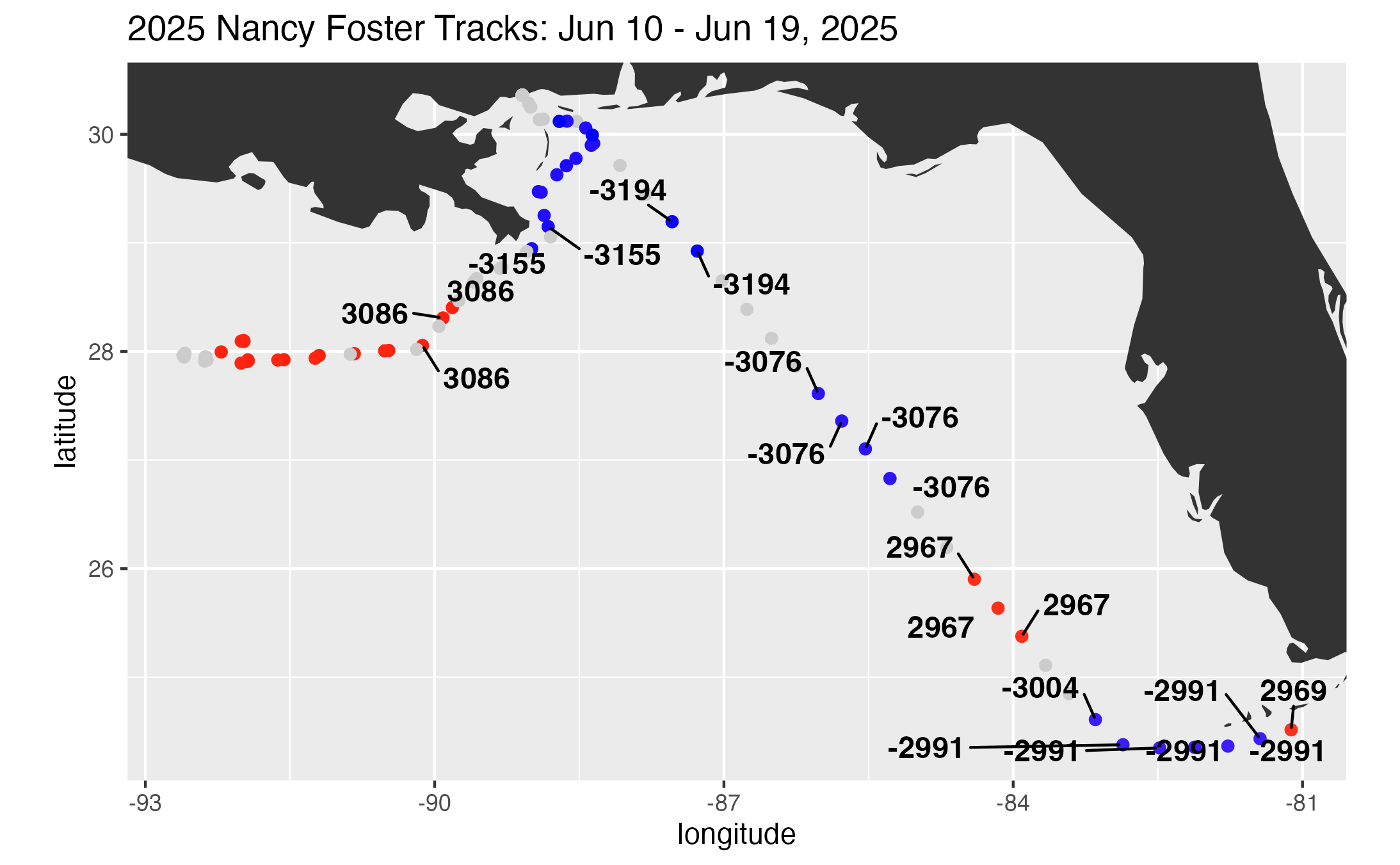
Exploring the MESI & MUNSTER eddy datasets
This code analyzes the eddy field along a June 2025 Gulf cruise track using satellite-derived sea level anomalies, MESI, MUNSTER eddy datasets, and underway data from NOAA Ship Nancy Foster. It first creates regional maps of SSH, EKE, MESI, and eddy locations, then overlays EKE, MESI, and eddy IDs along the cruise track.