Matchup Satellite data to track locations
history | Modified July 2024
Objective
This tutorial will demonstrate how to extract satellite data around a set of points defined by longitude, latitude, and time coordinates from an animal telemetry tag that was acquired from the Animal Telemetry Network (https://ioos.noaa.gov/project/atn/).
The tutorial demonstrates the following techniques
- Importing track data in csv file to data frame
- Plotting the latitude/longitude points onto a map
- Using rerddapXtraco function to extract satellite data from an ERDDAP data server along a track
- Plotting the satellite data onto a map
Datasets used in this exercise
Chlorophyll a concentration, the European Space Agency’s Ocean Colour Climate Change Initiative (OC-CCI) Monthly dataset v6.0
We’ll use the European Space Agency’s OC-CCI product (https://climate.esa.int/en/projects/ocean-colour/) to obtain chlorophyll data. This is a merged product combining data from many ocean color sensors to create a long time series (1997-present).
Yellowfin tuna telemetry track data
Marine protected areas (MPAs) in pelagic regions is also called Blue Water. The Palmyra Bluewater Research (PBR) project seeks to understand the impact of MPAs on species and ecosystems by tracking at-sea movements of ten marine animal species at Palmyra Atoll (part of the U.S. Pacific Remote Islands Marine National Monument). All data were being collected from adult individuals between May 2022 and June 2023. They can be accessed via the Animal Telemetry Network (ATN) data portal for the PBR project under “Project Data”: (https://portal.atn.ioos.us/?ls=861Wqpd2#metadata/1f877c4c-7b50-49f5-be86-3354664e0cff/project/files)
The yellowfin tuna geolocation data is developed as part of the PBR project. This example track used in the tutorial is from May 2022 to November 2022. The track data has been previously downloaded, extracted, and stored in the data folder of this training module.
Install required packages and load libraries
# Function to check if pkgs are installed, and install any missing pkgs
pkgTest <- function(x)
{
  if (!require(x,character.only = TRUE))
  {
    install.packages(x,dep=TRUE,repos='http://cran.us.r-project.org')
    if(!require(x,character.only = TRUE)) stop(x, " :Package not found")
  }
}


# Create list of required packages
list.of.packages <- c("rerddap", "plotdap", "parsedate", "ggplot2", "rerddapXtracto",
                       "date", "maps", "mapdata", "RColorBrewer","viridis", "stringr")

# Create list of installed packages
pkges = installed.packages()[,"Package"]

# Install and load all required pkgs
for (pk in list.of.packages) {
  pkgTest(pk)
}
Download animal track data from the ATN website
The data you need for this exercise are already in the GitHub repository
The following step are show you how to download the data yourself
ATN Portal
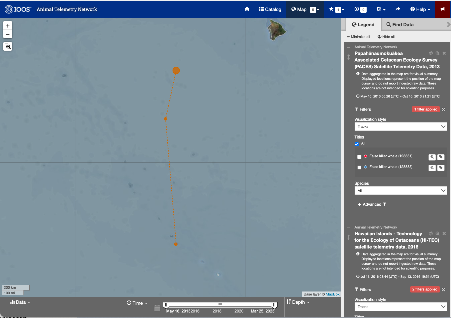
- Follow the link to the ATN website: https://portal.atn.ioos.us/?ls=O6vlufm7#map
- On the right navigational panel, look for the “Palmyra Bluewater Research (PBR) Megafauna Movement Ecology Project, 2022-2023” tab.
- Within the tab, scroll to find the telemetry tag labeled “Yellowfin tuna (233568)”.
- Click the search icon (maginifying glass) label next to the label to zoom into the area the area of the animal track.
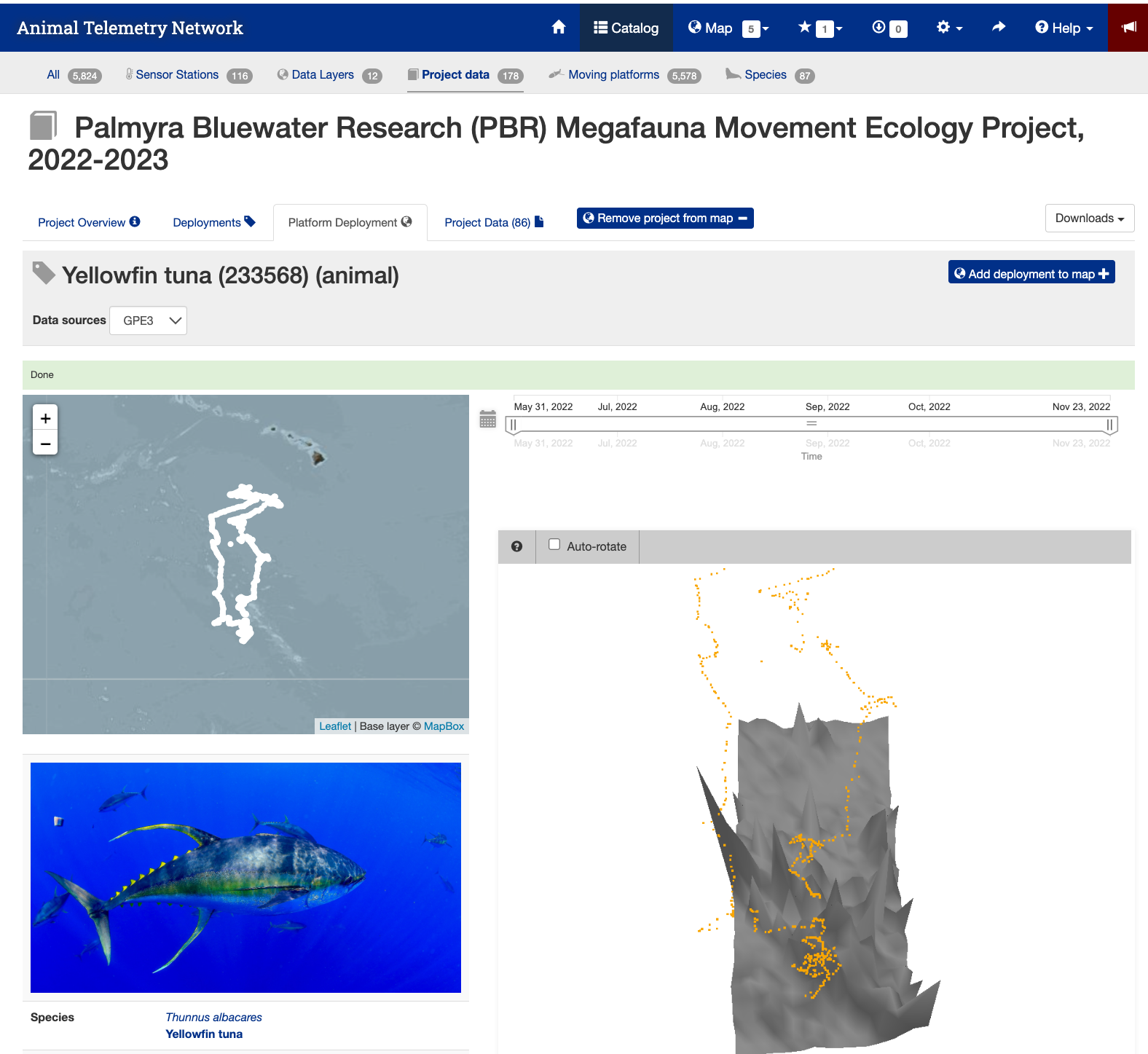
Detail page for the Yellowfin tuna (233568)
- Next click the tag icon to the right of the search icon.
- This page shows you details about the animal and the track.
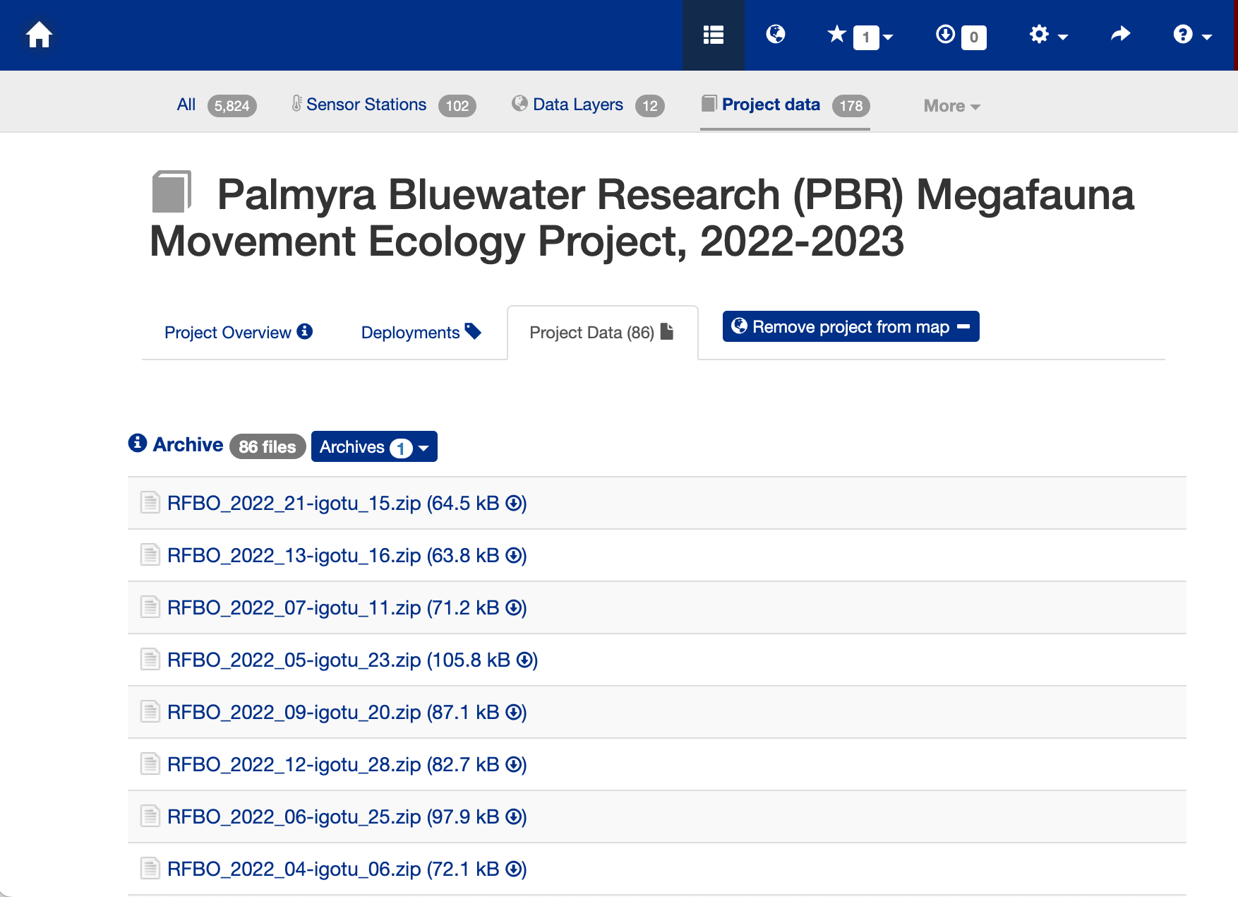
Data Download Page
- Press the “Project Data” tab near the top of the webpage to bring up the data file list.
- Search for the animal id number (233568).
- Click on the link “THUALB_2022_04-PTT_233568.zip (8.6 MB)” to download the data.
The Downloaded Data File
- The download will be a zip file. You will need to unzip it.
- The unzipped file folder contains many ancillary data files, but the one you are looking for is the CSV file (THUALB_2022_04-233568-4-GPE3.csv).
- You don’t have to move this file into the data folder for this exercise. It is already there.
- But if you download the file for a different animal track you would need to put the CSV file into the folder.
Import the track data into a data frame
# Import csv file into a data frame
file = "../data/THUALB_2022_04-233568-5-GPE3.csv"
pre_tuna_df <- read.csv(file, skip = 5)

# Show 3 rows from the data frame
head(pre_tuna_df, 3)
## DeployID Ptt Date Most.Likely.Latitude
## 1 THUALB_2022_04 233568 31-May-2022 19:00:00 5.875
## 2 THUALB_2022_04 233568 01-Jun-2022 00:00:00 5.875
## 3 THUALB_2022_04 233568 01-Jun-2022 04:56:15 5.850
## Most.Likely.Longitude Observation.Type Observed.SST Satellite.SST
## 1 -162.125 User NA NA
## 2 -162.100 None NA NA
## 3 -161.975 Light - Dusk NA NA
## Observed.Depth Bathymetry.Depth Observation.LL..MSS. Observation.Score
## 1 NA NA NA 68.60585
## 2 NA NA NA NA
## 3 144 2908 NA 43.16747
## Sunrise Sunset
## 1
## 2 01-Jun-2022 16:33:04 02-Jun-2022 04:59:36
## 3# Convert longitudes to 0~360 (Re-center map to the dateline)
pre_tuna_df['Most.Likely.Longitude'] <- pre_tuna_df['Most.Likely.Longitude'] + 360
# Show converted data frame
head(pre_tuna_df, 3)## DeployID Ptt Date Most.Likely.Latitude
## 1 THUALB_2022_04 233568 31-May-2022 19:00:00 5.875
## 2 THUALB_2022_04 233568 01-Jun-2022 00:00:00 5.875
## 3 THUALB_2022_04 233568 01-Jun-2022 04:56:15 5.850
## Most.Likely.Longitude Observation.Type Observed.SST Satellite.SST
## 1 197.875 User NA NA
## 2 197.900 None NA NA
## 3 198.025 Light - Dusk NA NA
## Observed.Depth Bathymetry.Depth Observation.LL..MSS. Observation.Score
## 1 NA NA NA 68.60585
## 2 NA NA NA NA
## 3 144 2908 NA 43.16747
## Sunrise Sunset
## 1
## 2 01-Jun-2022 16:33:04 02-Jun-2022 04:59:36
## 3Convert date string to a date object
pre_tuna_df$Date <- as.Date(pre_tuna_df$Date, format = "%d-%b-%Y")
head(pre_tuna_df)
## DeployID Ptt Date Most.Likely.Latitude Most.Likely.Longitude
## 1 THUALB_2022_04 233568 2022-05-31 5.875 197.875
## 2 THUALB_2022_04 233568 2022-06-01 5.875 197.900
## 3 THUALB_2022_04 233568 2022-06-01 5.850 198.025
## 4 THUALB_2022_04 233568 2022-06-01 5.900 198.025
## 5 THUALB_2022_04 233568 2022-06-01 5.900 198.025
## 6 THUALB_2022_04 233568 2022-06-01 5.900 198.025
## Observation.Type Observed.SST Satellite.SST Observed.Depth Bathymetry.Depth
## 1 User NA NA NA NA
## 2 None NA NA NA NA
## 3 Light - Dusk NA NA 144 2908
## 4 None NA NA NA NA
## 5 SST 28.2 28.32458 1 2908
## 6 Light - Dawn NA NA 112 2908
## Observation.LL..MSS. Observation.Score Sunrise
## 1 NA 68.60585
## 2 NA NA 01-Jun-2022 16:33:04
## 3 NA 43.16747
## 4 NA NA
## 5 NA 76.62995
## 6 NA 54.92253
## Sunset
## 1
## 2 02-Jun-2022 04:59:36
## 3
## 4
## 5
## 6Bin multiple observations from each day into daily mean values
The track data has multiple longitude/latitude/time points for each date. That temporal resolution is much higher than the daily and month satellite datasets that are available. So, let’s reduce the multiple daily values for the animal track data to a single value for each day. The code below creates a new dataframe that bins data for each date and calculates the mean for selected columns.
library(dplyr)
tuna_df <- pre_tuna_df %>% group_by(Date) %>% summarize(Most.Likely.Latitude = mean(Most.Likely.Latitude),
                                         Most.Likely.Longitude = mean(Most.Likely.Longitude),
                                         Satellite.SST = mean(Satellite.SST, na.rm=TRUE),
                                         Observed.SST = mean(Observed.SST, na.rm=TRUE),
                                         Observed.Depth = mean(Observed.Depth, na.rm=TRUE),
                                         Bathymetry.Depth = mean(Bathymetry.Depth, na.rm=TRUE),
                                         )

tuna_df
## # A tibble: 177 × 7
## Date Most.Likely.Latitude Most.Likely.Longitude Satellite.SST
## <date> <dbl> <dbl> <dbl>
## 1 2022-05-31 5.88 198. NaN
## 2 2022-06-01 5.88 198 28.3
## 3 2022-06-02 5.92 198. 28.3
## 4 2022-06-03 5.92 198. 28.3
## 5 2022-06-04 5.98 198. 28.3
## 6 2022-06-05 6.11 198. 28.4
## 7 2022-06-06 6.28 198. 28.3
## 8 2022-06-07 6.45 197. 28.3
## 9 2022-06-08 6.51 197. 28.2
## 10 2022-06-09 6.78 197. 28.2
## # ℹ 167 more rows
## # ℹ 3 more variables: Observed.SST <dbl>, Observed.Depth <dbl>,
## # Bathymetry.Depth <dbl>Plot the track on a map
# Download world map
mapWorld <- map_data("world", wrap=c(0,360))

# Map tuna tracks
ggplot(tuna_df, aes(Most.Likely.Longitude,Most.Likely.Latitude)) +
  geom_path(group=1)+
  geom_point(aes(x=Most.Likely.Longitude,y=Most.Likely.Latitude), pch=1, size=2 )+
  geom_point(aes(x=Most.Likely.Longitude[1],y=Most.Likely.Latitude[1]),fill="green", shape=24, size=3)+
  geom_point(aes(x=Most.Likely.Longitude[length(Most.Likely.Longitude)],y=Most.Likely.Latitude[length(Most.Likely.Latitude)]), shape=22, size=3, fill="red")+
  geom_polygon(data = mapWorld, aes(x=long, y = lat, group = group)) +
  coord_fixed(xlim = c(180,220),ylim = c(0,26))+
  labs(x="Longitude (deg)", y="Latitude (deg)", title="Yellowfin Tuna Track with start (green) and end location (red)")+
  theme(plot.title=element_text(hjust=0.5), aspect.ratio=0.6)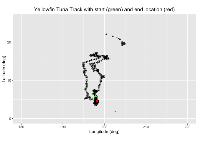
In this exercise, two different ways of extracting data from ERDDAP data server along a track of xyt points are demonstrated:
- Using the rerddapXtracto package which was written specifically for this task
- For those who want to know what goes on “under the hood”, we will show how to manually construct ERDDAP data-request URLs to download the data.
Extracting XYT data using the rerddapXtracto package
We will use the `rxtracto function of the rerddapXtracto package, which was written to simplify data extraction from ERDDAP servers.
Let’s use data from the monthly product of the OC-CCI datasets.
Ideally, we would work with daily data since we have one location per day. But chlorophyll data are severely affected by clouds (i.e. lots of missing data), so you might need to use weekly or even monthly data to get sufficient non-missing data. We will start with the monthly chl-a data since it contains fewer data gaps.
The ERDDAP URL to the monthly product is below:
https://oceanwatch.pifsc.noaa.gov/erddap/griddap/esa-cci-chla-monthly-v6-0
A note on dataset selection
We have preselected the dataset because we know it will work with this exercise. If you were selecting datasets on your own, you would want to check out the dataset to determine if its spatial and temporal coverages are suitable for your application. Following the link above you will find:
The latitude range is -89.97916 to 89.97916 and the longitude range is 0.020833 to 359.97916, which covers the track latitude range of 23.72 to 41.77 and longitude range of 175.86 to 248.57.
The time range is 1997-09-04 to 2023-12-01 (at the day of this writing), which covers the track time range of 2022-05-30 to 2023-01-18.
You should also note the name of the variable you will be downloading. For this dataset it is “chlor_a”
# Set dataset ID
dataset <- 'esa-cci-chla-monthly-v6-0'

# Get data information from ERDDAP server
dataInfo <- rerddap::info(dataset, url= "https://oceanwatch.pifsc.noaa.gov/erddap")
Examine metadata
rerddap::info returns the metadata of the requested dataset. We can first understand the attributes dataInfo includes then examine each attribute.
# Display the metadata
dataInfo
## <ERDDAP info> esa-cci-chla-monthly-v6-0
## Base URL: https://oceanwatch.pifsc.noaa.gov/erddap
## Dataset Type: griddap
## Dimensions (range):
## time: (1997-09-04T00:00:00Z, 2023-12-01T00:00:00Z)
## latitude: (-89.97916666666666, 89.97916666666667)
## longitude: (0.020833333333314386, 359.97916666666663)
## Variables:
## chlor_a:
## Units: mg m-3
## chlor_a_log10_bias:
## chlor_a_log10_rmsd:
## MERIS_nobs_sum:
## MODISA_nobs_sum:
## OLCI_A_nobs_sum:
## OLCI_B_nobs_sum:
## SeaWiFS_nobs_sum:
## total_nobs_sum:
## VIIRS_nobs_sum:# Display data attributes
names(dataInfo)## [1] "variables" "alldata" "base_url"# Examine attribute: variables
dataInfo$variables## variable_name data_type actual_range
## 1 chlor_a float
## 2 chlor_a_log10_bias float
## 3 chlor_a_log10_rmsd float
## 4 MERIS_nobs_sum float
## 5 MODISA_nobs_sum float
## 6 OLCI_A_nobs_sum float
## 7 OLCI_B_nobs_sum float
## 8 SeaWiFS_nobs_sum float
## 9 total_nobs_sum float
## 10 VIIRS_nobs_sum float# Distribute attributes of dataInfo$alldata
names(dataInfo$alldata)## [1] "NC_GLOBAL" "time" "latitude"
## [4] "longitude" "chlor_a" "MERIS_nobs_sum"
## [7] "MODISA_nobs_sum" "OLCI_A_nobs_sum" "OLCI_B_nobs_sum"
## [10] "SeaWiFS_nobs_sum" "VIIRS_nobs_sum" "chlor_a_log10_bias"
## [13] "chlor_a_log10_rmsd" "total_nobs_sum"Extract data using the rxtracto function
First we need to define the bounding box within which to search for coordinates. The rxtracto function allows you to set the size of the box used to collect data around the track points using the xlen and ylen arguments. The values for xlen and ylen are in degrees. For our example, we can use 0.2 degrees for both arguments. Note: You can also submit vectors for xlen and ylen, as long as they are the same length as xcoord, ycoord, and tcoord if you want to set a different search radius around each track point.
# Set the variable we want to extract data from:
parameter <- 'chlor_a'

# Set xlen, ylen to 0.2 degree
xlen <- 0.2
ylen <- 0.2

# Create date column using year, month and day in a format ERDDAP will understand (eg. 2008-12-15)
#tuna_df$date <-as.Date(tuna_df$Date, format = "%d-%b-%Y")

# Get variables x, y, t coordinates from tuna track data
xcoords <- tuna_df$Most.Likely.Longitude
ycoords <- tuna_df$Most.Likely.Latitude
tcoords <- tuna_df$Date

# Extract satellite data using x, y, t coordinates from tuna track data
chl_track <- rxtracto(dataInfo,
                  parameter=parameter,
                  xcoord=xcoords, ycoord=ycoords,
                  tcoord=tcoords, xlen=xlen, ylen=ylen)
Check the output of the rxtracto function
# Check all variables extracted using rxtracto
str(chl_track)
## List of 13
## $ mean chlor_a : num [1:177] 0.35 0.34 0.349 0.367 0.276 ...
## $ stdev chlor_a : num [1:177] 0.373 0.372 0.373 0.407 0.154 ...
## $ n : int [1:177] 36 36 36 30 25 36 30 36 36 30 ...
## $ satellite date : chr [1:177] "2022-06-01T00:00:00Z" "2022-06-01T00:00:00Z" "2022-06-01T00:00:00Z" "2022-06-01T00:00:00Z" ...
## $ requested lon min: num [1:177] 198 198 198 198 198 ...
## $ requested lon max: num [1:177] 198 198 198 198 198 ...
## $ requested lat min: num [1:177] 5.78 5.79 5.83 5.83 5.88 ...
## $ requested lat max: num [1:177] 5.97 5.98 6.02 6.02 6.08 ...
## $ requested z min : logi [1:177] NA NA NA NA NA NA ...
## $ requested z max : logi [1:177] NA NA NA NA NA NA ...
## $ requested date : chr [1:177] "2022-05-31" "2022-06-01" "2022-06-02" "2022-06-03" ...
## $ median chlor_a : num [1:177] 0.235 0.227 0.232 0.236 0.232 ...
## $ mad chlor_a : num [1:177] 0.017 0.0148 0.0172 0.0151 0.0192 ...
## - attr(*, "row.names")= chr [1:177] "1" "2" "3" "4" ...
## - attr(*, "class")= chr [1:2] "list" "rxtractoTrack"
## - attr(*, "base_url")= chr "https://oceanwatch.pifsc.noaa.gov/erddap/"
## - attr(*, "datasetid")= chr "esa-cci-chla-monthly-v6-0"rxtracto computes statistics using all the pixels found in the search radius around each track point.
Plotting the results using plotTrack
We will use the “plotTrack” function to plot the results. “plotTrack” is a function of the “rerddapXtracto” package designed specifically to plot the results of the “rxtracto” function. It provides an easy way to make a quick plot, however it’s not very customizable.
# Plot tracks with color: algae specifically designed for chlorophyll
plotTrack(chl_track, xcoords, ycoords, tcoords, size=3, plotColor = 'viridis')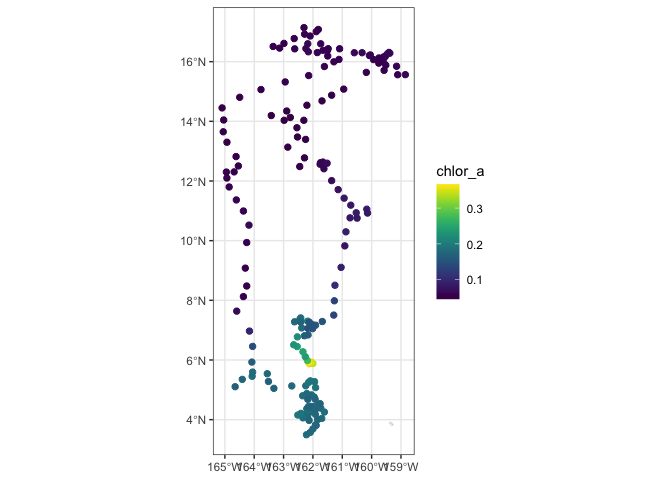
Animating the track
One of the nice features of the “plotTrack” function is that it is very easy to make an animation of the track data. This will take a minute to run. It creates an animated gif that will display in the Rstudio viewer window once the encoding to gif is done. Note: this works with but doesn’t require the latest versions of R Studio or rerddapXtracto package (e.g., it works with R Studio Version 2023.12.1+402 and rerddapXtracto version 1.1.5).
# Animate tracks

make180 <- function(lon) {
    ind <- which(lon > 180)
    lon[ind] <- lon[ind] - 360
   return(lon)
}

plotTrack(chl_track,
          make180(xcoords),
          ycoords, tcoords,
          plotColor = 'viridis',
          animate = TRUE,
          cumulative = TRUE)
## # A tibble: 177 × 7
## format width height colorspace matte filesize density
## <chr> <int> <int> <chr> <lgl> <int> <chr>
## 1 gif 672 480 sRGB TRUE 0 72x72
## 2 gif 672 480 sRGB TRUE 0 72x72
## 3 gif 672 480 sRGB TRUE 0 72x72
## 4 gif 672 480 sRGB TRUE 0 72x72
## 5 gif 672 480 sRGB TRUE 0 72x72
## 6 gif 672 480 sRGB TRUE 0 72x72
## 7 gif 672 480 sRGB TRUE 0 72x72
## 8 gif 672 480 sRGB TRUE 0 72x72
## 9 gif 672 480 sRGB TRUE 0 72x72
## 10 gif 672 480 sRGB TRUE 0 72x72
## # ℹ 167 more rowsPlotting the results using ggplot
Create a data frame with the tuna track and the output of rxtracto
If we to do an customization of the plot, its better to plot the data using ggplot. We will first create a data frame that contains longitudes and latitudes from the tuna and associated satellite chlor-a values.
# Create a data frame of coords from tuna and chlor_a values
new_df <- as.data.frame(cbind(xcoords, ycoords,
                              chl_track$`requested lon min`,
                              chl_track$`requested lon max`,
                              chl_track$`requested lat min`,
                              chl_track$`requested lon max`,
                              chl_track$`mean chlor_a`)
                        )

# Set variable names
names(new_df) <- c("Lon",
                   "Lat",
                   "Matchup_Lon_Lower",
                   "Matchup_Lon_Upper",
                   "Matchup_Lat_Lower",
                   "Matchup_Lat_Upper",
                   "Chlor_a")

write.csv(new_df, "tuna_matchup_df.csv")
Plot using ggplot
# Import world map
mapWorld <- map_data("world", wrap=c(0,360))

# Draw the track positions with associated chlora values
ggplot(new_df) +
  geom_point(aes(Lon,Lat,color=log(Chlor_a))) +
  geom_polygon(data = mapWorld, aes(x=long, y = lat, group = group)) +
  coord_fixed(xlim = c(180,220),ylim = c(0,26)) +
  scale_color_viridis(discrete = FALSE) +
  labs(x="Longitude (deg)", y="Latitude (deg)", title="Yellowfin Tuna Track with chlor-a values") +
  theme(plot.title=element_text(hjust=0.5))
Extracting XYT data by constructing the URL data requests manually
First we need to set up the ERDDAP URL using the datasets ID and the name of the variable we are interested in. Note that we are requesting the data as .csv
data_url = "https://oceanwatch.pifsc.noaa.gov/erddap/griddap/esa-cci-chla-monthly-v6-0.csv?chlor_a"
For a refresher of how to construct an ERDDAP data-request URL, please review the ERDDAP tutorial “04-Erddapurl.md” at the following link: https://github.com/coastwatch-training/CoastWatch-Tutorials/blob/main/ERDDAP-basics/lessons/
# Set erddap address
erddap_base_url <- "https://oceanwatch.pifsc.noaa.gov/erddap/griddap/esa-cci-chla-monthly-v6-0.csv?chlor_a"

# Get longitude and latitude from tuna track data
lon <- tuna_df$Most.Likely.Longitude
lat <- tuna_df$Most.Likely.Latitude

# Get time from tuna track data and convert into ERDDAP date format
dates2 <- as.Date(tuna_df$Date, format = "%d-%b-%Y")

# Initatilize tot variable where data will be downloaded to
tot <- rep(NA, 4)

# Loop through each tuna track data
for (i in 1:dim(tuna_df)[1]) {

  # follow the progress of the loop
  cat("\014")
  cat(" Loop ", i, " of ", dim(tuna_df)[1])

  # Create erddap URL by adding lat, lon, dates of each track point
   url <-  paste(erddap_base_url,
                 "[(", dates2[i], "):1:(", dates2[i],
                 ")][(", lat[i], "):1:(", lat[i],
                 ")][(", lon[i], "):1:(", lon[i], ")]", sep = "")

   # Request and load satelite data from ERDDAP
   new <- read.csv(url, skip=2, header = FALSE)

   # Append the data
   tot <- rbind(tot, new)

}
##
Loop 1 of 177
Loop 2 of 177
Loop 3 of 177
Loop 4 of 177
Loop 5 of 177
Loop 6 of 177
Loop 7 of 177
Loop 8 of 177
Loop 9 of 177
Loop 10 of 177
Loop 11 of 177
Loop 12 of 177
Loop 13 of 177
Loop 14 of 177
Loop 15 of 177
Loop 16 of 177
Loop 17 of 177
Loop 18 of 177
Loop 19 of 177
Loop 20 of 177
Loop 21 of 177
Loop 22 of 177
Loop 23 of 177
Loop 24 of 177
Loop 25 of 177
Loop 26 of 177
Loop 27 of 177
Loop 28 of 177
Loop 29 of 177
Loop 30 of 177
Loop 31 of 177
Loop 32 of 177
Loop 33 of 177
Loop 34 of 177
Loop 35 of 177
Loop 36 of 177
Loop 37 of 177
Loop 38 of 177
Loop 39 of 177
Loop 40 of 177
Loop 41 of 177
Loop 42 of 177
Loop 43 of 177
Loop 44 of 177
Loop 45 of 177
Loop 46 of 177
Loop 47 of 177
Loop 48 of 177
Loop 49 of 177
Loop 50 of 177
Loop 51 of 177
Loop 52 of 177
Loop 53 of 177
Loop 54 of 177
Loop 55 of 177
Loop 56 of 177
Loop 57 of 177
Loop 58 of 177
Loop 59 of 177
Loop 60 of 177
Loop 61 of 177
Loop 62 of 177
Loop 63 of 177
Loop 64 of 177
Loop 65 of 177
Loop 66 of 177
Loop 67 of 177
Loop 68 of 177
Loop 69 of 177
Loop 70 of 177
Loop 71 of 177
Loop 72 of 177
Loop 73 of 177
Loop 74 of 177
Loop 75 of 177
Loop 76 of 177
Loop 77 of 177
Loop 78 of 177
Loop 79 of 177
Loop 80 of 177
Loop 81 of 177
Loop 82 of 177
Loop 83 of 177
Loop 84 of 177
Loop 85 of 177
Loop 86 of 177
Loop 87 of 177
Loop 88 of 177
Loop 89 of 177
Loop 90 of 177
Loop 91 of 177
Loop 92 of 177
Loop 93 of 177
Loop 94 of 177
Loop 95 of 177
Loop 96 of 177
Loop 97 of 177
Loop 98 of 177
Loop 99 of 177
Loop 100 of 177
Loop 101 of 177
Loop 102 of 177
Loop 103 of 177
Loop 104 of 177
Loop 105 of 177
Loop 106 of 177
Loop 107 of 177
Loop 108 of 177
Loop 109 of 177
Loop 110 of 177
Loop 111 of 177
Loop 112 of 177
Loop 113 of 177
Loop 114 of 177
Loop 115 of 177
Loop 116 of 177
Loop 117 of 177
Loop 118 of 177
Loop 119 of 177
Loop 120 of 177
Loop 121 of 177
Loop 122 of 177
Loop 123 of 177
Loop 124 of 177
Loop 125 of 177
Loop 126 of 177
Loop 127 of 177
Loop 128 of 177
Loop 129 of 177
Loop 130 of 177
Loop 131 of 177
Loop 132 of 177
Loop 133 of 177
Loop 134 of 177
Loop 135 of 177
Loop 136 of 177
Loop 137 of 177
Loop 138 of 177
Loop 139 of 177
Loop 140 of 177
Loop 141 of 177
Loop 142 of 177
Loop 143 of 177
Loop 144 of 177
Loop 145 of 177
Loop 146 of 177
Loop 147 of 177
Loop 148 of 177
Loop 149 of 177
Loop 150 of 177
Loop 151 of 177
Loop 152 of 177
Loop 153 of 177
Loop 154 of 177
Loop 155 of 177
Loop 156 of 177
Loop 157 of 177
Loop 158 of 177
Loop 159 of 177
Loop 160 of 177
Loop 161 of 177
Loop 162 of 177
Loop 163 of 177
Loop 164 of 177
Loop 165 of 177
Loop 166 of 177
Loop 167 of 177
Loop 168 of 177
Loop 169 of 177
Loop 170 of 177
Loop 171 of 177
Loop 172 of 177
Loop 173 of 177
Loop 174 of 177
Loop 175 of 177
Loop 176 of 177
Loop 177 of 177# Delete the first row (default column names)
tot <- tot[-1, ]
# Rename columns
names(tot) <- c("chlo_date", "matched_lat", "matched_lon", "matched_chl.m")
# Create data frame combining tuna track data and the chlo-a data
chl_track2 <- data.frame(tuna_df, tot)
# Write the data frame to csv file
write.csv(chl_track2, 'tuna-track-chl.m.csv', row.names = FALSE)Make a map of the data extracted using ggplot
# Draw the track positions with associated chlora values
ggplot(chl_track2) +
  geom_point(aes(Most.Likely.Longitude,Most.Likely.Latitude,color=log(matched_chl.m))) +
  geom_polygon(data = mapWorld, aes(x=long, y = lat, group = group)) +
  coord_fixed(xlim = c(180,220),ylim = c(0,26)) +
  scale_color_viridis(discrete = FALSE) +
  labs(x="Longitude (deg)", y="Latitude (deg)", title="Yellowfin Tuna Track with chlor-a values")+
  theme(plot.title=element_text(hjust=0.5))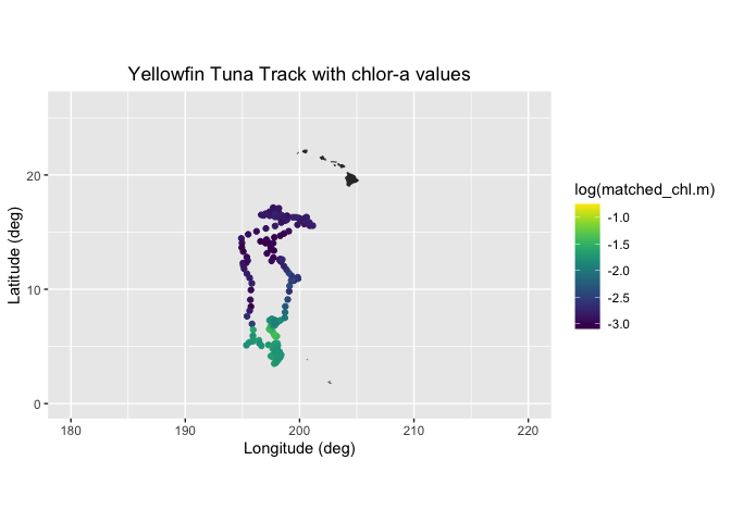
Plot histogram of chlorophyll
How do the chlorophyll values of the tuna track compare to values in the surrounding environment? Meaning does the tuna seem to have a preference for certain chlorophyll values? To look at this we will plot a histograms of the track chl valuesand those of the surrounding area.
First we will get a 3D block of chl data from the region and of the tuna track over the span of time the tuna was in that area. We will use the ‘xtracto_3d’ function of rerddapXtracto to get the data. This data call will take a few minutes.
chl_grid <- rxtracto_3D(dataInfo,
                  parameter=parameter,
                  xcoord=c(min(xcoords),max(xcoords)),
                  ycoord=c(min(ycoords),max(ycoords)),
                  tcoord=c(min(tcoords),max(tcoords)))

chl_area <- as.vector(chl_grid$chlor_a)

# remove NA values
chl_area <- chl_area[!is.na(chl_area)]

# vector or tuna chlorophyll

chl_tuna <- chl_track$`mean chlor_a`
Now we we plot histograms of all the chlorphyll values in the area, and those of the tuna track.
ggplot(as.data.frame(chl_area)) +
      geom_histogram(aes(x=chl_area,y=after_stat(density),color = "darkgray",fill='Area'),color='black', bins=50) +
      geom_histogram(data=as.data.frame(chl_tuna), aes(x=chl_tuna,y=after_stat(density),color='green', fill='Tuna'),color='black',bins=50, alpha=.4) +
      scale_x_continuous(limits = c(0,.9), expand = c(0, 0)) +
      scale_y_continuous(limits = c(0,15), expand = c(0, 0)) +
      labs(x='Chlorophyll values',y='Density') +
      theme_bw() +
      scale_fill_manual(values=c("darkgray","green"),'')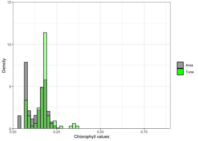
Exercise 1:
Repeat the steps above with a different satellite dataset. For example, extract sea surface temperature data using the following dataset: https://coastwatch.pfeg.noaa.gov/erddap/griddap/nesdisGeoPolarSSTN5NRT_Lon0360.html \ This dataset is a different ERDDAP, so remember to change the base URL. \ Set the new dataset ID and variable name.
Exercise 2:
Go to an ERDDAP of your choice, find a dataset of interest, generate the URL, copy it and edit the script above to run a match up on that dataset. To find other ERDDAP servers, you can use this search engine: http://erddap.com/ \ This dataset will likely be on a different ERDDAP, so remember to change the base URL. \ Set the new dataset ID and variable name. \ Check the metadata to make sure the dataset covers the spatial and temporal range of the track dataset.
Optional
Repeat the steps above with a daily version of the OC-CCI dataset to see how cloud cover can reduce the data you retrieve. https://coastwatch.pfeg.noaa.gov/erddap/griddap/pmlEsaCCI60OceanColorDaily_Lon0360.html