Matchup Satellite data to track locations

history | Modified Feb 2026

Objective

This tutorial will demonstrate how to extract satellite data around a set of points defined by longitude, latitude, and time coordinates, like those produced by an animal telemetry tag, and ship track, or a glider track.

The tutorial demonstrates the following techniques

Importing track data in csv file to data frame
Plotting the latitude/longitude points onto a map
Using rerddapXtraco function to extract satellite data from an ERDDAP data server along a track
Plotting the satellite data onto a map
Subsetting and analyzing data for individual animals
Comparing satellite-derived environmental conditions across time

Datasets used

Chlorophyll a concentration, the European Space Agency’s Ocean Colour Climate Change Initiative (OC-CCI) Monthly dataset v6.0

We’ll use the European Space Agency’s OC-CCI product (https://climate.esa.int/en/projects/ocean-colour/) to obtain chlorophyll data. This is a merged product combining data from many ocean color sensors to create a long time series (1997-present).

Loggerhead turtle telemetry track data

The turtle was raised in captivity in Japan, then tagged and released on 05/04/2005 in the Central Pacific. Its tag transmitted for over 3 years and went all the way to the Southern tip of Baja California. This dataset has been subsampled to reduce the data requests needed for this tutorial from over 1200 to 25. The track data are stored in the data folder in this project folder.

Dusky shark satellite tag data

An extended example uses satellite tag data from dusky sharks provided by Chuck Bangley (Smithsonian Environmental Research Center). This dataset includes daily positions from multiple tagged individuals and demonstrates how the same ERDDAP extraction workflow can be applied to a different species and telemetry format. The shark example highlights additional steps such as data validation, subsetting individual animals, and comparing satellite-derived chlorophyll values across years.

Chlorophyll-a, Aqua MODIS, NPP, L3SMI, Global, 4km, Science Quality, 2003-present (8 Day Composite)

Install required packages and load libraries

# Function to check if pkgs are installed, and install any missing pkgs
pkgTest <- function(x)
{
  if (!require(x,character.only = TRUE))
  {
    install.packages(x,dep=TRUE,repos='http://cran.us.r-project.org')
    if(!require(x,character.only = TRUE)) stop(x, " :Package not found")
  }
}


# Create list of required packages
list.of.packages <- c("rerddap", "plotdap", "parsedate", "ggplot2", "rerddapXtracto",
                       "date", "maps", "mapdata", "RColorBrewer","viridis")

# Create list of installed packages
pkges = installed.packages()[,"Package"]

# Install and load all required pkgs
for (pk in list.of.packages) {
  pkgTest(pk)
}

Import the track data into a data frame

# Import csv file into a data frame
turtle_df <- read.csv("../data/25317_05_subsampled.dat")
# Show 3 rows from the data frame
head(turtle_df,3)

##   mean_lon mean_lat year month day
## 1 176.6194 32.67873 2005     5   4
## 2 175.8609 35.05773 2005     6  23
## 3 180.5926 40.40576 2005     8  12

Plot the track on a map

# Download world map
mapWorld <- map_data("world", wrap=c(0,360))

# Map turtle tracks
ggplot(turtle_df, aes(mean_lon,mean_lat)) +
  geom_path(group=1)+
  geom_point(aes(x=mean_lon,y=mean_lat), pch=1, size=2 )+
  geom_point(aes(x=mean_lon[1],y=mean_lat[1]),fill="green", shape=24, size=3)+
  geom_point(aes(x=mean_lon[length(mean_lon)],y=mean_lat[length(mean_lat)]), shape=22, size=3, fill="red")+
  geom_polygon(data = mapWorld, aes(x=long, y = lat, group = group)) + 
  coord_fixed(xlim = c(120,260),ylim = c(15,60))+
  labs(x="Longitude (deg)", y="Latitude (deg)", title="Turtle Track with start (green) and end location (red)")+
  theme(plot.title=element_text(hjust=0.5), aspect.ratio=1/2)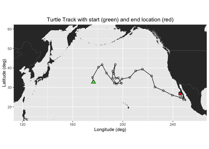

In this exercise, two different ways of extracting data from ERDDAP data server along a track of xyt points are demonstrated:

Using the rerddapXtracto package which was written specifically for this task
By manually constructing a URL with the data data request

Extracting XYT data using the rerddapXtracto package

We will use the `rxtracto function of the rerddapXtracto package, which was written to simplify data extraction from ERDDAP servers.

Let’s use data from the monthly product of the OC-CCI datasets.
The ERDDAP URL to the monthly product is below:
https://oceanwatch.pifsc.noaa.gov/erddap/griddap/esa-cci-chla-monthly-v6-0

A note on dataset selection
We have preselected the dataset because we know it will work with this exercise. If you were selecting datasets on your own, you would want to check out the dataset to determine if its spatial and temporal coverages are suitable for your application. Following the link above you will find:

The latitude range is -89.97916 to 89.97916 and the longitude range is 0.020833 to 359.97916, which covers the track latitude range of 23.72 to 41.77 and longitude range of 175.86 to 248.57.

The time range is 1997-09-04 to 2023-12-01 (at the day of this writing), which covers the track time range of 2005-05-04 to 2008-08-16.

You should also note the name of the variable you will be downloading. For this dataset it is “chlor_a”

# Set dataset ID
dataset <- 'esa-cci-chla-monthly-v6-0'

# Get data information from ERDDAP server
dataInfo <- rerddap::info(dataset, url= "https://oceanwatch.pifsc.noaa.gov/erddap")

Examine metadata

rerddap::info returns the metadata of the requested dataset. We can first understand the attributes dataInfo includes then examine each attribute.

# Display the metadata
dataInfo

## <ERDDAP info> esa-cci-chla-monthly-v6-0 
##  Base URL: https://oceanwatch.pifsc.noaa.gov/erddap 
##  Dataset Type: griddap 
##  Dimensions (range):  
##      time: (1997-09-04T00:00:00Z, 2023-12-01T00:00:00Z) 
##      latitude: (-89.97916666666666, 89.97916666666667) 
##      longitude: (0.020833333333314386, 359.97916666666663) 
##  Variables:  
##      chlor_a: 
##          Units: mg m-3 
##      chlor_a_log10_bias: 
##      chlor_a_log10_rmsd: 
##      MERIS_nobs_sum: 
##      MODISA_nobs_sum: 
##      OLCI_A_nobs_sum: 
##      OLCI_B_nobs_sum: 
##      SeaWiFS_nobs_sum: 
##      total_nobs_sum: 
##      VIIRS_nobs_sum:

# Display data attributes
names(dataInfo)

## [1] "variables" "alldata"   "base_url"

# Examine attribute: variables
dataInfo$variables

##         variable_name data_type actual_range
## 1             chlor_a     float             
## 2  chlor_a_log10_bias     float             
## 3  chlor_a_log10_rmsd     float             
## 4      MERIS_nobs_sum     float             
## 5     MODISA_nobs_sum     float             
## 6     OLCI_A_nobs_sum     float             
## 7     OLCI_B_nobs_sum     float             
## 8    SeaWiFS_nobs_sum     float             
## 9      total_nobs_sum     float             
## 10     VIIRS_nobs_sum     float

# Distribute attributes of dataInfo$alldata
names(dataInfo$alldata)

##  [1] "NC_GLOBAL"          "time"               "latitude"          
##  [4] "longitude"          "chlor_a"            "MERIS_nobs_sum"    
##  [7] "MODISA_nobs_sum"    "OLCI_A_nobs_sum"    "OLCI_B_nobs_sum"   
## [10] "SeaWiFS_nobs_sum"   "VIIRS_nobs_sum"     "chlor_a_log10_bias"
## [13] "chlor_a_log10_rmsd" "total_nobs_sum"

Extract data using the rxtracto function

First we need to define the bounding box within which to search for coordinates. The rxtracto function allows you to set the size of the box used to collect data around the track points using the xlen and ylen arguments. The values for xlen and ylen are in degrees. For our example, we can use 0.2 degrees for both arguments. Note: You can also submit vectors for xlen and ylen, as long as they are the same length as xcoord, ycoord, and tcoord if you want to set a different search radius around each track point.

# Set the variable we want to extract data from:
parameter <- 'chlor_a'

# Set xlen, ylen to 0.2 degree
xlen <- 0.2 
ylen <- 0.2

# Create date column using year, month and day in a format ERDDAP will understand (eg. 2008-12-15)
turtle_df$date <- as.Date(paste(turtle_df$year, turtle_df$month, turtle_df$day, sep="-"))

# Get variables x, y, t coordinates from turtle track data
xcoords <- turtle_df$mean_lon
ycoords <- turtle_df$mean_lat
tcoords <- turtle_df$date

# Extract satellite data using x, y, t coordinates from turtle track data
chl_track <- rxtracto(dataInfo, 
                  parameter=parameter, 
                  xcoord=xcoords, ycoord=ycoords, 
                  tcoord=tcoords, xlen=xlen, ylen=ylen)

Check the output of the rxtracto function

# Check all variables extracted using rxtracto
chl_track

## $`mean chlor_a`
##  [1] 0.26779765 0.12073122 0.30777924 0.31780368 0.28884829 0.36146353
##  [7] 0.22923882 0.11644071 0.09268904 0.05536651 0.18447913 0.22765385
## [13] 0.23869553 0.24669819 0.35838123 0.09624625 0.12024124 0.11400095
## [19] 0.10017463 0.09397742 0.08515869 0.06913812 0.14883095 0.51560753
## [25] 0.65806269
## 
## $`stdev chlor_a`
##  [1] 0.032191816 0.007231171 0.036716832 0.041052758 0.027952051 0.053364804
##  [7] 0.024394244 0.007282479 0.003880810 0.001490017 0.040774493 0.025363286
## [13] 0.014782180 0.013523678 0.036640145 0.004842596 0.004098601 0.003910613
## [19] 0.003537558 0.005928580 0.007001476 0.004942355 0.011980482 0.099209610
## [25] 0.149563991
## 
## $n
##  [1] 36 36 36 27 36 30 36 36 30 30 30 30 36 30 36 30 36 36 36 30 36 30 36 36 36
## 
## $`satellite date`
##  [1] "2005-05-01T00:00:00Z" "2005-07-01T00:00:00Z" "2005-08-01T00:00:00Z"
##  [4] "2005-10-01T00:00:00Z" "2005-12-01T00:00:00Z" "2006-01-01T00:00:00Z"
##  [7] "2006-03-01T00:00:00Z" "2006-05-01T00:00:00Z" "2006-06-01T00:00:00Z"
## [10] "2006-08-01T00:00:00Z" "2006-09-01T00:00:00Z" "2006-11-01T00:00:00Z"
## [13] "2007-01-01T00:00:00Z" "2007-02-01T00:00:00Z" "2007-04-01T00:00:00Z"
## [16] "2007-06-01T00:00:00Z" "2007-07-01T00:00:00Z" "2007-09-01T00:00:00Z"
## [19] "2007-11-01T00:00:00Z" "2007-12-01T00:00:00Z" "2008-02-01T00:00:00Z"
## [22] "2008-04-01T00:00:00Z" "2008-05-01T00:00:00Z" "2008-07-01T00:00:00Z"
## [25] "2008-08-01T00:00:00Z"
## 
## $`requested lon min`
##  [1] 176.5194 175.7609 180.4926 183.4102 186.8997 193.2152 198.9158 196.2679
##  [9] 194.2116 192.7545 193.9788 191.9444 191.6600 194.9631 199.2066 205.5050
## [17] 210.1805 215.6225 222.9073 225.5386 232.3064 239.4530 245.7716 248.4710
## [25] 245.6579
## 
## $`requested lon max`
##  [1] 176.7194 175.9609 180.6926 183.6102 187.0997 193.4152 199.1158 196.4679
##  [9] 194.4116 192.9545 194.1788 192.1444 191.8600 195.1631 199.4066 205.7050
## [17] 210.3805 215.8225 223.1073 225.7386 232.5064 239.6530 245.9716 248.6710
## [25] 245.8579
## 
## $`requested lat min`
##  [1] 32.57873 34.95773 40.30576 41.58480 37.26623 32.03793 32.01126 34.81224
##  [9] 34.59661 36.99175 41.66933 38.12796 34.63858 31.63964 34.24324 35.02771
## [17] 38.36083 39.23749 35.76793 30.08540 28.22859 25.88108 24.73662 23.62417
## [25] 26.68177
## 
## $`requested lat max`
##  [1] 32.77873 35.15773 40.50576 41.78480 37.46623 32.23793 32.21126 35.01224
##  [9] 34.79661 37.19175 41.86933 38.32796 34.83858 31.83964 34.44324 35.22771
## [17] 38.56083 39.43749 35.96793 30.28540 28.42859 26.08108 24.93662 23.82417
## [25] 26.88177
## 
## $`requested z min`
##  [1] NA NA NA NA NA NA NA NA NA NA NA NA NA NA NA NA NA NA NA NA NA NA NA NA NA
## 
## $`requested z max`
##  [1] NA NA NA NA NA NA NA NA NA NA NA NA NA NA NA NA NA NA NA NA NA NA NA NA NA
## 
## $`requested date`
##  [1] "2005-05-04" "2005-06-23" "2005-08-12" "2005-10-01" "2005-11-20"
##  [6] "2006-01-09" "2006-02-28" "2006-04-19" "2006-06-08" "2006-07-28"
## [11] "2006-09-16" "2006-11-05" "2006-12-25" "2007-02-13" "2007-04-04"
## [16] "2007-05-24" "2007-07-13" "2007-09-01" "2007-10-21" "2007-12-10"
## [21] "2008-01-29" "2008-03-19" "2008-05-08" "2008-06-27" "2008-08-16"
## 
## $`median chlor_a`
##  [1] 0.26985641 0.11935977 0.31413330 0.31312889 0.28226255 0.35456662
##  [7] 0.22596541 0.11711950 0.09256660 0.05540323 0.18355133 0.22467585
## [13] 0.24202415 0.24848759 0.34953472 0.09518800 0.11983451 0.11379882
## [19] 0.10012896 0.09296544 0.08735247 0.06766215 0.14883141 0.49834299
## [25] 0.67895702
## 
## $`mad chlor_a`
##  [1] 0.030100095 0.008344179 0.039171724 0.027213317 0.023952735 0.049566912
##  [7] 0.022928175 0.009027836 0.003463391 0.001267676 0.035848973 0.026539111
## [13] 0.016244819 0.011793729 0.035606685 0.003954114 0.002984454 0.002953619
## [19] 0.002999692 0.003767908 0.003242842 0.003565519 0.015092995 0.109981245
## [25] 0.133971250
## 
## attr(,"row.names")
##  [1] "1"  "2"  "3"  "4"  "5"  "6"  "7"  "8"  "9"  "10" "11" "12" "13" "14" "15"
## [16] "16" "17" "18" "19" "20" "21" "22" "23" "24" "25"
## attr(,"class")
## [1] "list"          "rxtractoTrack"

rxtracto computes statistics using all the pixels found in the search radius around each track point.

Plotting the results using plotTrack

We will use the “plotTrack” function to plot the results. “plotTrack” is a function of the “rerddapXtracto” package designed specifically to plot the results of the “rxtracto” function. It provides an easy way to make a quick plot, however it’s not very customizable.

# Plot tracks with color: algae specifically designed for chlorophyll
plotTrack(chl_track, xcoords, ycoords, tcoords, size=3, plotColor = 'viridis')

Animating the track

One of the nice features of the “plotTrack” function is that it is very easy to make an animation of the track data. This will take a minute to run. It creates an animated gif that will display in the Rstudio viewer window once the encoding to gif is done.

# Animate tracks

make180 <- function(lon) {
    ind <- which(lon > 180)
    lon[ind] <- lon[ind] - 360
   return(lon)
}

plotTrack(chl_track, make180(xcoords), ycoords, tcoords, plotColor = 'viridis',
                    animate = TRUE, cumulative = TRUE)

## # A tibble: 25 × 7
##    format width height colorspace matte filesize density
##    <chr>  <int>  <int> <chr>      <lgl>    <int> <chr>  
##  1 gif      672    480 sRGB       TRUE         0 72x72  
##  2 gif      672    480 sRGB       TRUE         0 72x72  
##  3 gif      672    480 sRGB       TRUE         0 72x72  
##  4 gif      672    480 sRGB       TRUE         0 72x72  
##  5 gif      672    480 sRGB       TRUE         0 72x72  
##  6 gif      672    480 sRGB       TRUE         0 72x72  
##  7 gif      672    480 sRGB       TRUE         0 72x72  
##  8 gif      672    480 sRGB       TRUE         0 72x72  
##  9 gif      672    480 sRGB       TRUE         0 72x72  
## 10 gif      672    480 sRGB       TRUE         0 72x72  
## # ℹ 15 more rows

Plotting the results using ggplot

Create a data frame with the turtle track and the output of rxtracto

If we to do an customization of the plot, its better to plot the dat ausing ggplot. We will first create a data frame that contains longitudes and latitudes from the turtle and associated satellite chlor-a values.

# Create a data frame of coords from turtle and chlor_a values 
new_df <- as.data.frame(cbind(xcoords, ycoords,  
                              chl_track$`requested lon min`, 
                              chl_track$`requested lon max`, 
                              chl_track$`requested lat min`, 
                              chl_track$`requested lon max`,  
                              chl_track$`mean chlor_a`))

# Set variable names
names(new_df) <- c("Lon", "Lat", "Matchup_Lon_Lower", "Matchup_Lon_Upper", "Matchup_Lat_Lower", "Matchup_Lat_Upper",  "Chlor_a")
write.csv(new_df, "matchup_df.csv")

Plot using ggplot

# Import world map
mapWorld <- map_data("world", wrap=c(0,360))

# Draw the track positions with associated chlora values
ggplot(new_df) +
  geom_point(aes(Lon,Lat,color=log(Chlor_a))) +
  geom_polygon(data = mapWorld, aes(x=long, y = lat, group = group)) + 
  coord_fixed(xlim = c(120,260),ylim = c(15,60)) +
  scale_color_viridis(discrete = FALSE) +
  labs(x="Longitude (deg)", y="Latitude (deg)", title="Turtle Track with chlor-a values")+
  theme(plot.title=element_text(hjust=0.5))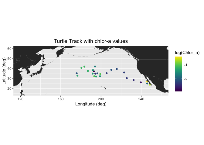

Extracting XYT data by constructing the URL data requests manually

First we need to set up the ERDDAP URL using the datasets ID and the name of the variable we are interested in. Note that we are requesting the data as .csv

data_url = "https://oceanwatch.pifsc.noaa.gov/erddap/griddap/aqua_chla_1d_2018_0.csv?chlor_a"

Ideally, we would work with daily data since we have one location per day. But chlorophyll data is severely affected by clouds (i.e. lots of missing data), so you might need to use weekly or even monthly data to get sufficient non-missing data. We will start with the monthly chl-a data since it contains fewer gaps.

# Set erddap address
erddap <- "https://oceanwatch.pifsc.noaa.gov/erddap/griddap/aqua_chla_monthly_2018_0.csv?chlor_a"

# Get longitude and latitude from turtle track data
lon <- turtle_df$mean_lon
lat <- turtle_df$mean_lat

# Get time from turtle track data and convert into ERDDAP date format
dates <- mdy.date(turtle_df$month,turtle_df$day,turtle_df$year)
dates2 <- format(as.Date(dates), "%Y-%m-%d")

# Initatilize tot variable where data will be downloaded to
tot <- rep(NA, 4)

# Loop through each turtle track data
for (i in 1:dim(turtle_df)[1]) {

   # Create erddap URL by adding lat, lon, dates of each track point 
   url <-  paste(erddap, "[(", dates2[i], "):1:(", dates2[i], ")][(", lat[i], "):1:(", lat[i], ")][(", lon[i], "):1:(", lon[i], ")]", sep = "")  
   
   # Request and load satelite data from ERDDAP
   new <- read.csv(url, skip=2, header = FALSE) 
   
   # Append the data
   tot <- rbind(tot, new)   
}

# Delete the first row (default column names)
tot <- tot[-1, ]

# Rename columns
names(tot) <- c("chlo_date", "matched_lat", "matched_lon", "matched_chl.m")

# Create data frame combining turtle track data and the chlo-a data
chl_track2 <- data.frame(turtle_df, tot)

# Write the data frame to csv file
write.csv(chl_track2, 'turtle-track-chl.m.csv', row.names = FALSE)

Make a map of the data extracted using the second method

# Draw the track positions with associated chlora values
ggplot(chl_track2) +
  geom_point(aes(mean_lon,mean_lat,color=log(matched_chl.m))) +
  geom_polygon(data = mapWorld, aes(x=long, y = lat, group = group)) + 
  coord_fixed(xlim = c(120,260),ylim = c(15,60)) +
  scale_color_viridis(discrete = FALSE) +
  labs(x="Longitude (deg)", y="Latitude (deg)", title="Turtle Track with chlor-a values")+
  theme(plot.title=element_text(hjust=0.5))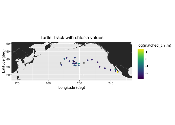

Plot histogram of chlorophyll

How do the chlorophyll values of the turtle track compare to values in the surrounding environment? Meaning does the turtle seem to have a preference for certain chlorophyll values? To look at this we will plot a histograms of the track chl valuesand those of the surrounding area.

First we will get a 3D block of chl data from the region and of the turtle track over the span of time the turtle was in that area. We will use the ‘xtracto_3d’ function of rerddapXtracto to get the data. This data call will take a few minutes.

chl_grid <- rxtracto_3D(dataInfo, 
                  parameter=parameter, 
                  xcoord=c(min(xcoords),max(xcoords)), 
                  ycoord=c(min(ycoords),max(ycoords)), 
                  tcoord=c(min(tcoords),max(tcoords)))

chl_area <- as.vector(chl_grid$chlor_a) 

# remove NA values 
chl_area <- chl_area[!is.na(chl_area)]

# vector or turtle chlorophyll 

chl_turtle <- chl_track$`mean chlor_a`

Now we we plot histograms of all the chlorphyll values in the area, and those of the turtle track. Since we subset the turtletrack, and only have 25 points for this subsampopled dataset the turtle histogram isn’t as useful as it would be with a larger dataset.

ggplot(as.data.frame(chl_area)) + 
      geom_histogram(aes(x=chl_area,y=after_stat(density),color = "darkgray",fill='Area'),color='black', bins=50) + 
      geom_histogram(data=as.data.frame(chl_turtle), aes(x=chl_turtle,y=after_stat(density),color='green', fill='Turtle'),color='black',bins=50, alpha=.4) + 
      scale_x_continuous(limits = c(0,.9), expand = c(0, 0)) + 
      scale_y_continuous(limits = c(0,15), expand = c(0, 0)) +
      labs(x='Chlorophyll values',y='Density') + 
      theme_bw() + 
      scale_fill_manual(values=c("darkgray","green"),'')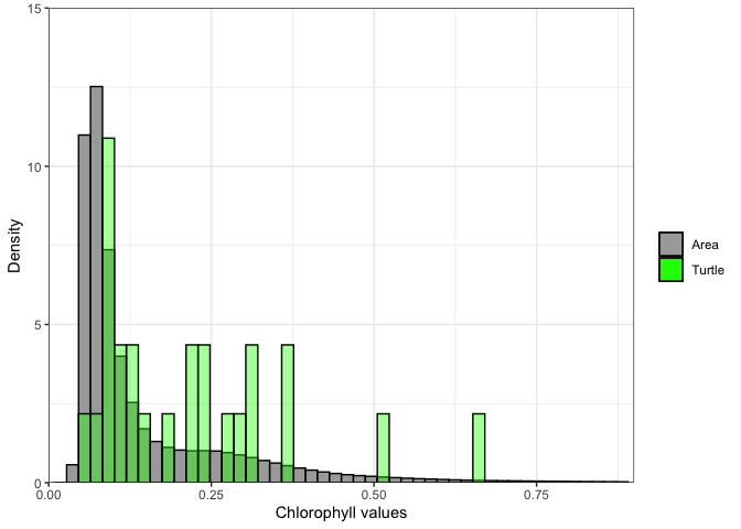

Exercise 1:

Repeat the steps above with a different dataset. For example, extract sea surface temperature data using the following dataset: https://coastwatch.pfeg.noaa.gov/erddap/griddap/nesdisGeoPolarSSTN5NRT_Lon0360.html \ This dataset is a different ERDDAP, so remember to change the base URL. \ Set the new dataset ID and variable name.

Exercise 2:

Go to an ERDDAP of your choice, find a dataset of interest, generate the URL, copy it and edit the script above to run a match up on that dataset. To find other ERDDAP servers, you can use this search engine: http://erddap.com/ \ This dataset will likely be on a different ERDDAP, so remember to change the base URL. \ Set the new dataset ID and variable name. \ Check the metadata to make sure the dataset covers the spatial and temporal range of the track dataset.

Optional

Repeat the steps above with a daily version of the OC-CCI dataset to see how cloud cover can reduce the data you retrieve. https://coastwatch.pfeg.noaa.gov/erddap/griddap/pmlEsaCCI60OceanColorDaily_Lon0360.html

Match satellite chlorophyll to Dusky shark telemetry

In this example, we extend the techniques demonstrated above to a different type of animal telemetry dataset: satellite-tagged Dusky sharks. While the workflow is conceptually the same, this example highlights several additional considerations that commonly arise when working with real telemetry data.

Data note: These dusky shark data were collected and provided by Dr. Chuck Bangley (Smithsonian Environmental Research Center). For details, see:

Bangley, C.W., et al. (2020) Identifying Important Juvenile Dusky Shark Habitat in the Northwest Atlantic Ocean Using Acoustic Telemetry and Spatial Modeling. Marine and Coastal Fisheries, 12:348–363. DOI: 10.1002/mcf2.10120

Import and validate shark tag data

We load the Dusky shark tag data from a CSV file and perform a few basic checks to ensure the data are ready for analysis.

# Dusky shark tag data from Chuck Bangley (SERC)
infile <- file.path("DuskyDaily_NOAAclass_sortedTransmitterDate.csv")

if (!file.exists(infile)) {
  stop("Tag CSV not found: ", infile,
       "\nTip: put the CSV in your working directory or update `infile`.")
}

tagdata <- read.csv(infile, head = TRUE, sep = ",", stringsAsFactors = FALSE)

# Quick look
str(tagdata)

# Minimal column checks (same expected columns your script uses)
needed_cols <- c("Longitude", "Latitude", "Date", "Transmitter")
missing_cols <- setdiff(needed_cols, names(tagdata))
if (length(missing_cols) > 0) {
  stop("Missing required columns in tag CSV: ", paste(missing_cols, collapse = ", "))
}

Extract coordinates and format dates for ERDDAP

Extract the lat and lon values from the shark tag data and prepare the time information for use with ERDDAP. The rxtracto function requires coordinates to be supplied as a separate lon, lat, and time vectors.

xcoord <- tagdata$Longitude
ycoord <- tagdata$Latitude

# Convert m/d/YYYY -> YYYY-mm-dd (rxtracto expects character dates like this)
tcoord_chr <- as.character(as.Date(tagdata$Date, "%m/%d/%Y"))

# Optional: catch date parse failures (NA)
if (any(is.na(tcoord_chr))) {
  stop("Some dates could not be parsed with format '%m/%d/%Y'.\n",
       "Check the Date column (example: 12/31/2018).")
}

Retrieve and examine ERDDAP dataset metadata

Using the rerrdap::info() function, we query ERDDAP server for metadata describing the selected dataset.

url <- "https://coastwatch.pfeg.noaa.gov/erddap/"
dataset <- "erdMH1chla8day"

# Alternates (using WCN ERDDAP server):
# dataset <- "nesdisVHNSQchlaWeekly"          # Suomi-NPP VIIRS weekly chlorophyll, global 4km
# dataset <- "pmlEsaCCI50OceanColorMonthly"   # OC-CCI Chlorophyll, Monthly

# If you encounter an error reading the nc file, clear the rerddap cache:
# rerddap::cache_delete_all(force = TRUE)

dataInfo <- rerddap::info(dataset, url = url)
dataInfo

Extract satellite data along the track using `rxtracto`

Extract satellite-derived chlorophyll values at each shark tag location using the rxtracto function from the rerddapXtracto package. Satellite data are rarely available at an exact point in space, so rxtracto averages all satellite grid cells within a user-defined search radius around each track location. Here, we use a search window on 0.2° in both lon and lat. This spatial averaging helps account for differences in satellite resolution and small uncertainties in tag position.

parameter <- "chlorophyll"  # Chlorophyll, Aqua MODIS
# Alternate:
# parameter <- "chlor_a"     # Chlorophyll, Suomi-NPP VIIRS

# Some satellite datasets have an altitude dimension.
# If the dataInfo shows an altitude dimension, then zcoord must be included.
zcoord <- rep(0., length(xcoord))

# Search radius in degrees: satellite cells within +/- xlen/ylen are averaged
xlen <- 0.2
ylen <- 0.2

weekly_chl <- rxtracto(
  dataInfo,
  parameter = parameter,
  xcoord = xcoord, ycoord = ycoord,
  tcoord = tcoord_chr,
  xlen = xlen, ylen = ylen
)

# Save extracted values
write.csv(weekly_chl, "weekly_chl_rxtracto.csv", row.names = FALSE)

Visualize chlorophyll along the track

We use plotTrack to create a quick-look map of chlorophyll values along the sharks’ track.

# PlotTrack may not show the image in some environments.
# If so, uncomment these lines to save a PNG:
# png(file="chl_data_vals_at_shark_tag_locations.png")
plotTrack(weekly_chl, xcoord, ycoord, tcoord_chr, plotColor = "algae")
# dev.off()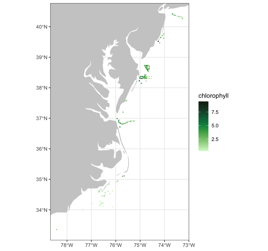

Combine track coordinates with extracted chlorophyll values

We create a tidy data frame that combines the shark tag locations with the corresponding satellie-derived chlorophyll values extracted using rxtracto.

alltags <- data.frame(
  x = xcoord,
  y = ycoord,
  dataval = weekly_chl$`mean chlorophyll`
)

# Alternate: Chlorophyll, Suomi-NPP VIIRS
# alltags <- data.frame(x = xcoord, y = ycoord, dataval = weekly_chl$`mean chlor_a`)

mapWorld <- map_data("world")

Select a single shark and plot

We subset the full dataset to focus on a single shark, identified by its transmitter ID. We use ggplot to create a map showing the selected shark’s track locations colored by the satellite-derived chlorophyll concentration.

transm <- tagdata$Transmitter
shark1 <- transm[1]          # selects the first value from transm
shark1                       # displays the transmitter number
shark1_index <- which(transm == shark1)

single_shark <- data.frame(
  x_shark = alltags$x[shark1_index],
  y_shark = alltags$y[shark1_index],
  dataval_shark = alltags$dataval[shark1_index]
)

# Zoom bounds for this shark 
maplonmax <- max(single_shark$x_shark)
maplonmin <- min(single_shark$x_shark)
maplatmax <- max(single_shark$y_shark)
maplatmin <- min(single_shark$y_shark)

mapplot_shark1 <- ggplot(single_shark) +
  geom_point(aes(x_shark, y_shark, color = dataval_shark), size = 2.) +
  geom_polygon(data = mapWorld, aes(x = long, y = lat, group = group), fill = "grey80") +
  coord_cartesian(xlim = c(maplonmin, maplonmax), ylim = c(maplatmin, maplatmax)) +
  scale_color_gradientn(colours = brewer.pal(n = 8, name = "YlGn"),
                        name = expression("Chlorophyll (mg m"^{-3}*")")) +
  labs(x = "", y = "") +
  ggtitle("Mean chl-a values for dusky shark #1 ")

mapplot_shark1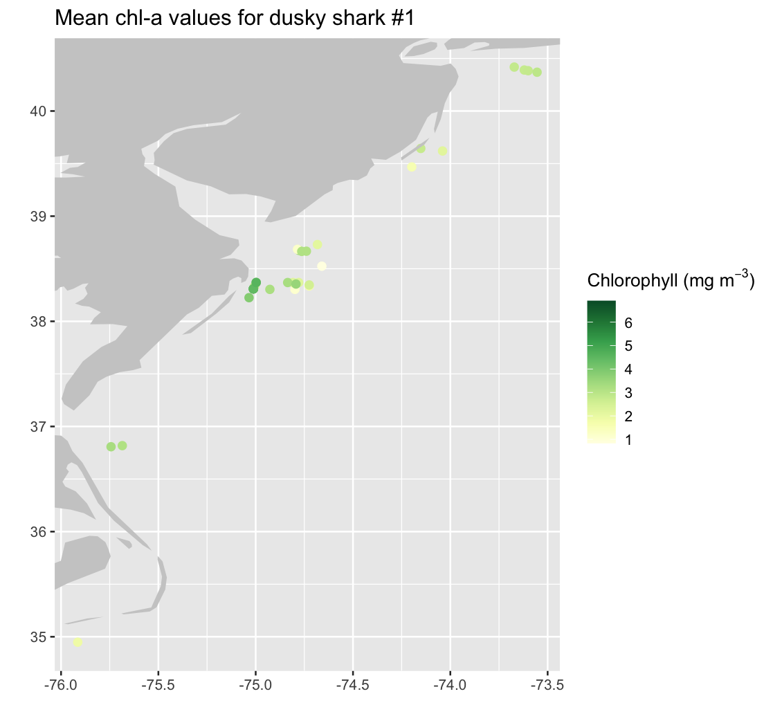

Add track segments to connect consecutive shark locations

Draw line segments to connect consecutive shark tag locations, creating a continuous movement track. Because a track with N location points contains N-1 movement segments, we construct a separate start and end coordinate vectors for each segment.

# Start/end points for N-1 line segments (same as your approach)
start_lon <- single_shark$x_shark[1:(length(single_shark$x_shark) - 1)]
start_lat <- single_shark$y_shark[1:(length(single_shark$y_shark) - 1)]
end_lon   <- single_shark$x_shark[2:length(single_shark$x_shark)]
end_lat   <- single_shark$y_shark[2:length(single_shark$y_shark)]

str(start_lon)

nseg <- length(start_lon)

mapplot_shark1_tracks <- mapplot_shark1 +
  geom_segment(
    data = as.data.frame(single_shark$dataval_shark[1:nseg]),
    aes(x = start_lon, y = start_lat, xend = end_lon, yend = end_lat)
  )

mapplot_shark1_tracks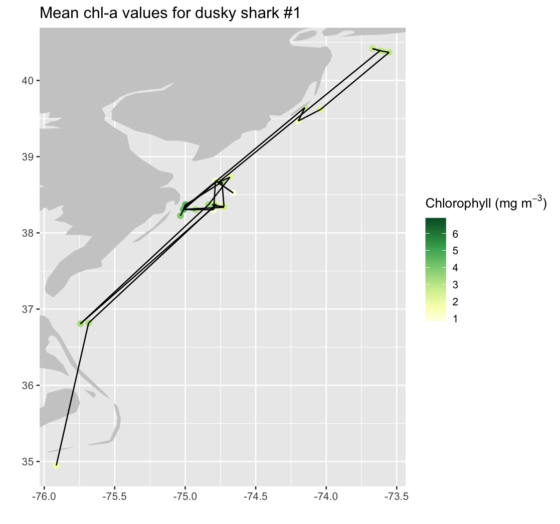

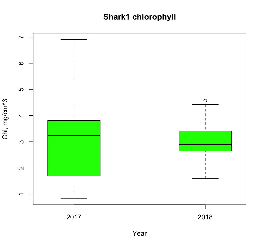
Compare chlorophyll values across years for a single shark

We add date information to the single-shark dataset and use it to examine how satellite-derived chlorophyll values vary across different years of the shark’s track. The data are subset by year allowing, us to separate observations from 2017 and 2018 for comparison. We then visualize these year-specific chlorophyll distributions using a boxplot.

date_shark <- tcoord_chr[shark1_index]
single_shark$date_shark <- date_shark

shark1_2017 <- subset(single_shark, format(as.Date(date_shark), "%Y") == 2017)
shark1_2018 <- subset(single_shark, format(as.Date(date_shark), "%Y") == 2018)

print(shark1_2017)
print(shark1_2018)

boxplot(
  shark1_2017$dataval_shark, shark1_2018$dataval_shark,
  main = "Shark1 chlorophyll",
  names = c("2017", "2018"),
  col = c("green"),
  xlab = "Year",
  ylab = "Chl, mg/cm^3",
  at = c(1, 3)  # draws boxplots at positions 1,3 with a space in the middle
)