Virtual Buoy example
history | Updated September 2023
NOAA PolarWatch distributes gridded and tabular oceanographic data for polar regions. Satellite data include geospatial information and most of them are in geographical coordinates (latitude and longitude). PolarWatch satellite data are often projected using Polar Stereographic Projections in x and y coordinates.
Objective
This tutorial will demonstrate how to plot a polar stereographic projected data on a projected map, and to add another dataset with geographical coordinates (latitude and longitude) onto the map.
The tutorial demonstrates the following techniques
- Accessing satellite data from ERDDAP
- Making a projected map
- Adding projected data
- Adding geographical data
Datasets used
Sea Ice Concentration, NOAA/NSIDC Climate Data Record V4, Northern Hemisphere, 25km, Science Quality, 1978-Present, Monthly
This dataset includes sea ice concentration data from the northern hemisphere, and is produced by the NOAA/NSIDC using the Climate Data Record algorithm. The resolution is 25km, meaning each grid in this data set represents a value that covers a 25km by 25km area. The dataset is avaialble from the NOAA PolarWatch Catalog.
Polar bear tracking data
For the demonstrative purpose of adding a dataset in geographical coords (lat, lon) to the projected map, GPS data for a polar bear track were used. More information about the data can be found at https://borealisdata.ca/file.xhtml?fileId=151017&version=1.0
R Packages
- ncdf4 (reading data and metadata in netCDF format)
- ggplot2, RColorBrewer, scales (mapping)
- reshape2 (data manipulation)
- rgdal (projection)
Install required packages
# Function to check if pkgs are installed, install missing pkgs, and load
pkgTest <- function(x)
{
if (!require(x,character.only = TRUE))
{
install.packages(x,dep=TRUE,repos='http://cran.us.r-project.org')
if(!require(x,character.only = TRUE)) stop(x, " :Package not found")
}
}
list.of.packages <- c("rgdal","sp", "ggplot2" ,"ncdf4", "RColorBrewer", "scales", "reshape2")
# create list of installed packages
pkges = installed.packages()[,"Package"]
for (pk in list.of.packages) {
pkgTest(pk)
}
# download the sea ice data NetCDF file
seaice_url <- "https://polarwatch.noaa.gov/erddap/griddap/nsidcG02202v4nhmday.nc?cdr_seaice_conc_monthly[(2022-12-01T00:00:00Z):1:(2022-12-01T00:00:00Z)][(4851137.11):1:(-4850758.92)][(-3850000.0):1:(3750000.0)]"
sea_ice_data_nc <- download.file(seaice_url, destfile="../data/sea_ice_data.nc", mode='wb')
# file open
seaice <- nc_open('../data/sea_ice_data.nc')
# print metadata
#print(seaice)
# get data into r variables
xgrid <- ncvar_get(seaice, "xgrid")
ygrid <- ncvar_get(seaice, "ygrid")
sic <- ncvar_get(seaice, "cdr_seaice_conc_monthly") #lat and lon
fillvalue <- ncatt_get(seaice, "cdr_seaice_conc_monthly", "_FillValue") #checkout fill value for missing data points
# close
nc_close(seaice)
# create dataframe
sicd <- expand.grid(xgrid=xgrid, ygrid=ygrid)
sicd$sic <- array(sic, dim(xgrid)*dim(ygrid))
# exclude fillvalue
sicd$sic[sicd$sic > 2] <- NA
# map sea ice concentration
ggplot(data = sicd, aes(x = xgrid, y = ygrid, fill=sic) ) +
geom_tile() +
coord_fixed(ratio = 1) +
scale_y_continuous(labels=comma) +
scale_x_continuous(labels=comma) +
scale_fill_gradientn(colours=rev(brewer.pal(n = 3, name = "Blues")),na.value="tan") +
ggtitle("Sea Ice Concentration on Polar Steregraphic projection")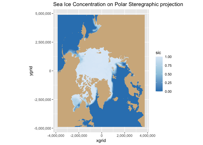 ### Adding Polar bear track data onto the polar stereographic projection
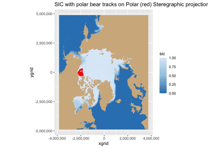
# read csv polar bear track data
polartrack <- read.csv("../data/PB_Argos.csv")
polarB <- polartrack[polartrack$QualClass=="B",]

# specify coordinate columns
coordinates(polarB) <- c("Lon", "Lat")

# set data crs to 4326
proj4string(polarB) <-CRS("+init=epsg:4326")

# transform the data crs from EPSG:4326 to EPSG: 3413
polar.3413 <- spTransform(polarB, CRS("+init=epsg:3413"))

# for ggplot, convert spatial data to data.frame
polar.3413.df<-data.frame(polar.3413)
names(polar.3413.df)[names(polar.3413.df)=="Lon"]<-"x"
names(polar.3413.df)[names(polar.3413.df)=="Lat"]<-"y"
Combine the sea ice concentration data and the polar bear tracking data
ggplot(data = sicd, aes(x = xgrid, y = ygrid) ) +
        geom_tile(aes(fill=sic)) +
       coord_fixed(ratio = 1) +
       scale_y_continuous(labels = comma) +
       scale_x_continuous(labels = comma) +
       scale_fill_gradientn(colours=rev(brewer.pal(n = 3, name = "Blues")),na.value="tan")+
       ggtitle("SIC with polar bear tracks on Polar (red) Steregraphic projection")+
      geom_point(data=polar.3413.df, aes(x=x, y=y), color="red", size=0.5)