Subset data in polar stereographic projection using a shape file fr

Updated September 2024

The tutorial demonstrates the following techniques

Download sea ice satellite data from the PolarWatch ERDDAP data server
Import geographical features of Lake Iliamna from a shapefile
Transform data from one projection to another
Subset the satellite data for Lake Iliamna
Visualize data in different projection

Data Used

World Lake shape data

The world lake shapefile can be downloaded from ArcGIS Hub at https://hub.arcgis.com, and is also available in the resource/ directory of this tutorial folder. The file includes geographical features of all world lakes. For this exercise, only the features of Lake Illemna will be used.

IMS Snow and Ice Analysis, Arctic, 4km, 2004 - Present, Daily (PolarWatch Preview)

The IMS dataset includes daily snow and ice coverage data for the Arctic with a 4-km resolution, available starting from 2004. The values in the dataset are categorical, representing five categories: 0 for areas outside the coverage zone, 1 for open water, 2 for land without snow, 3 for sea ice or lake ice, and 4 for snow-covered land. Data with a 1-km resolution are also available. Please contact us for more information.

Load packages

knitr::opts_chunk$set(
  echo = TRUE,
  fig.path = "images/",
  warning = FALSE, message = FALSE
)

# Function to check if pkgs are installed, install missing pkgs, and load

pkgTest <- function(x)
{
  if (!require(x,character.only = TRUE))
  {
    install.packages(x,dep=TRUE,repos='http://cran.us.r-project.org')
    if(!require(x,character.only = TRUE)) stop(x, " :Package not found")
  }
}

list.of.packages <- c("sp", "ggplot2" , "rerddap", "RColorBrewer", "scales", "reshape2")

# create list of installed packages
pkges = installed.packages()[,"Package"]
for (pk in list.of.packages) {
  pkgTest(pk)
}

library(terra)
library(sf)
library(ggplot2)
library(rerddap)

Load IMS Sea ice data from ERDDAP


pw_url = "https://polarwatch.noaa.gov/erddap/"
dataset_id = "usnic_ims_4km"
var_name = "IMS_Surface_Values"
dat_info <- info(datasetid = dataset_id, url = pw_url)
dat_info

Subset and extract ims data

dat <- griddap(dat_info,  time = c('2019-11-01','2019-11-01'), fields = var_name)
ims <- dat$data

Visualize the IMS satellite data

# Visualize the data (warning: this takes awhile to )
ggplot(data = ims, aes(x = x, y = y, fill=IMS_Surface_Values)) +
         geom_tile() + 
         coord_fixed(ratio = 1) + 
         scale_y_continuous() + 
         scale_x_continuous() +
         scale_fill_gradientn(colours=rev(brewer.pal(n = 3, name = "Blues")),na.value="tan") +
         ggtitle("IMS Data")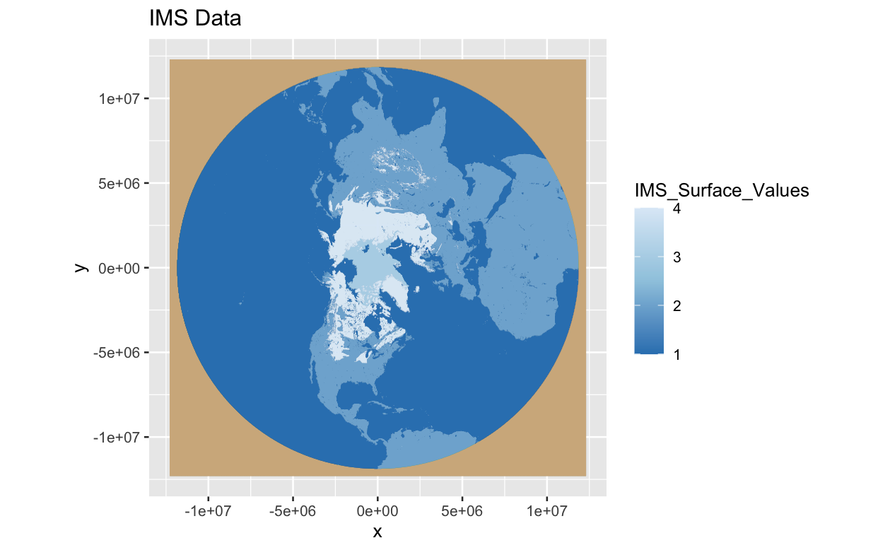

Convert IMS data to raster S4 object


# ensure numeric (rerddap often returns list columns)
ims$x <- as.numeric(unlist(ims$x))
ims$y <- as.numeric(unlist(ims$y))
ims[[var_name]] <- as.numeric(unlist(ims[[var_name]]))

# create raster from xyz explicitly
ims_ras <- terra::rast(ims[, c("x", "y", var_name)], type = "xyz")

# IMS 4km grid is Polar Stereographic (proj4 from NSIDC IMS user guide)
ims_proj4 <- "+proj=stere +lat_0=90 +lat_ts=60 +lon_0=-80 +k=1 +x_0=0 +y_0=0 +a=6378137 +b=6356257 +units=m +no_defs"
terra::crs(ims_ras) <- ims_proj4


# get CRS as an sf object for st_transform
data_crs <- sf::st_crs("EPSG:3857")
# plot the raster data
plot(ims_ras)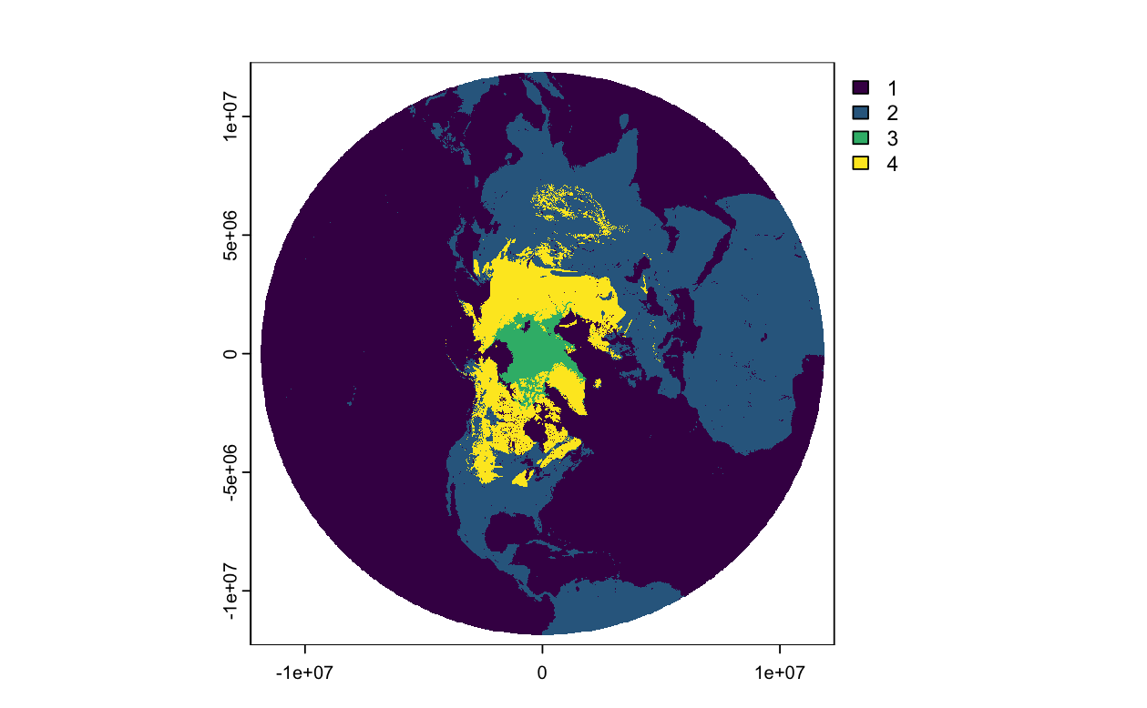

Load the lake shapefile

# Set directory path for shapefile
dir_path <- '../resources/Iliamna/Iliamna.shp'


# Load the shape file
shapes <- st_read(dsn = dir_path)

# View
print(shapes)

# Get boundary coordinates for Lake Iliamna
lake_shp <- shapes[shapes$Lake_name == "Iliamna", ]
ggplot(data = lake_shp) +
  geom_sf() +
  theme_minimal() +
  labs(title = "Lake Iliamna", 
       caption = "Source: shapefile")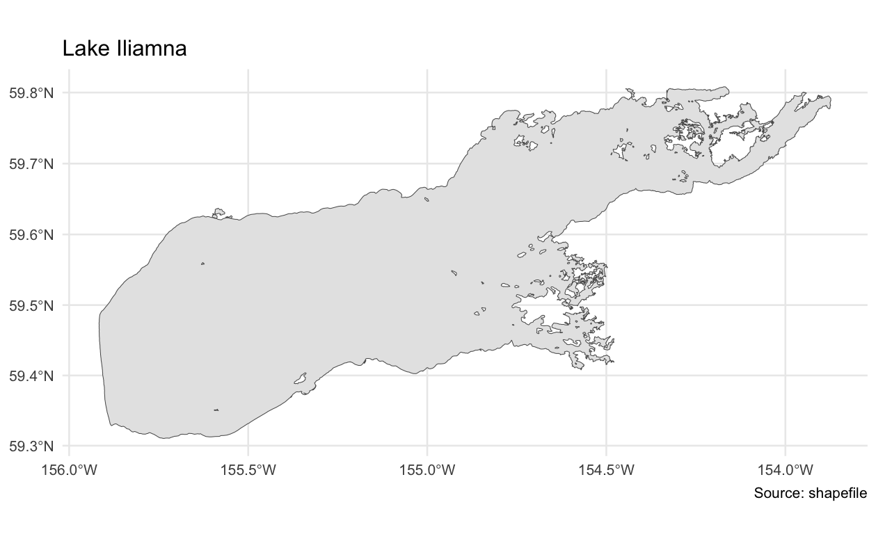

Convert the lake shape to raster S4 object


shapes_polar <- sf::st_transform(lake_shp, sf::st_crs(ims_proj4))
lake_ras <- terra::vect(shapes_polar)
plot(lake_ras, border = "red")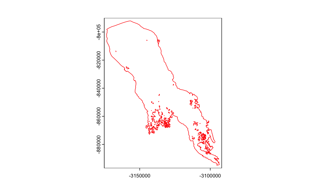

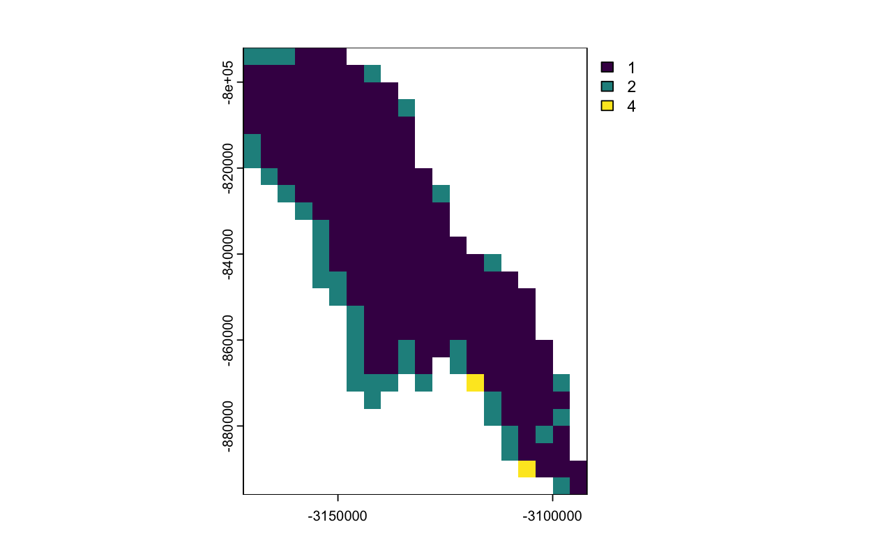
Crop the IMS data


# crop to the bounding box of the lake
cropped_lake <- crop(ims_ras, lake_ras)

# mask data with the lake shape
masked_lake <- mask(cropped_lake, lake_ras)
plot(masked_lake)