Define a marine habitat
notebook filename | define_marine_habitat.Rmd
Context
The TurleWatch project investigated the overlap between loggerhead sea turtles habitat and fishing effort of the Hawaii-based shallow-set longline fishery in the Pacific Ocean north of the Hawaiian Islands. That fishery, which targets swordfish, used to experience high levels of bycatch of loggerhead turtles. Considerable changes in gear and operations lowered bycatch rate and the TurtleWatch product was designed as a tool to advise fishermen on areas to avoid to limit bycatch.
Research results indicated that 50% of interactions occurred between 17.5°C and 18.5°C.
Objective
Here we will draw the 17.5 and 18.5ºC temperature contours on a map of satellite sea surface temperature.
The tutorial demonstrates the following techniques
- Using the xtracto_3D function to extract data from a rectangular area
- Masking a data array
- Plotting maps using plotBBox and ggplot
Datasets used
CoralTemp Sea Surface Temperature product from the NOAA Coral Reef Watch program. The NOAA Coral Reef Watch (CRW) daily global 5km Sea Surface Temperature (SST) product, also known as CoralTemp, shows the nighttime ocean temperature measured at the surface. The SST scale ranges from -2 to 35 °C. The CoralTemp SST data product was developed from two, related reanalysis (reprocessed) SST products and a near real-time SST product. Spanning January 1, 1985 to the present, the CoralTemp SST is one of the best and most internally consistent daily global 5km SST products available. More information about the product: https://coralreefwatch.noaa.gov/product/5km/index_5km_sst.php
Install required packages and load libraries
# Function to check if pkgs are installed, install missing pkgs, and load
pkgTest <- function(x)
{
  if (!require(x,character.only = TRUE))
  {
    install.packages(x,dep=TRUE,repos='http://cran.us.r-project.org')
    if(!require(x,character.only = TRUE)) stop(x, " :Package not found")
  }
}

list.of.packages <- c( "ncdf4", "rerddap", "plotdap", "RCurl",
                       "raster", "colorRamps", "maps", "mapdata",
                       "ggplot2", "RColorBrewer", "rerddapXtracto")

# create list of installed packages
pkges = installed.packages()[,"Package"]

for (pk in list.of.packages) {
  pkgTest(pk)
}
Select the Satellite Data
- Use the CoralTemp SST dataset (ID CRW_sst_v3_1) from the OceanWatch ERDDAP server (https://oceanwatch.pifsc.noaa.gov/erddap/index.html)
- Gather information about the dataset (metadata) using rerddap
- Display the information
# Let's look at the metadata


url = "https://oceanwatch.pifsc.noaa.gov/erddap/"
dataInfo <- rerddap::info('CRW_sst_v3_1',url=url)
parameter <- 'analysed_sst'dataInfo## <ERDDAP info> CRW_sst_v3_1
## Base URL: https://oceanwatch.pifsc.noaa.gov/erddap
## Dataset Type: griddap
## Dimensions (range):
## time: (1985-01-01T12:00:00Z, 2023-09-09T12:00:00Z)
## latitude: (-89.975, 89.975)
## longitude: (0.025, 359.975)
## Variables:
## analysed_sst:
## Units: degree_C
## sea_ice_fraction:
## Units: 1Get Satellite Data
- Select an area of the central North Pacific where the fishery operates: longitude range of 185 to 235 east and latitude range of 20 to 45 north
- Select a date in the first quarter of the year when bycatch typically occurs:
tcoord=c('2023-01-06', '2023-01-06')).tcoordneeds to be a vector even if we are pulling only one day of data.
# latitude and longitude of the vertices
ylim<-c(20,45)
xlim<-c(185,235)

# Extract the data
SST <- rxtracto_3D(dataInfo,xcoord=xlim,ycoord=ylim,parameter=parameter,
                   tcoord=c('2023-01-06','2023-01-06'))

# Drop command needed to reduce SST from a 3D variable to a 2D  one
SST$analysed_sst <- drop(SST$analysed_sst)
Make a quick plot using plotBBox
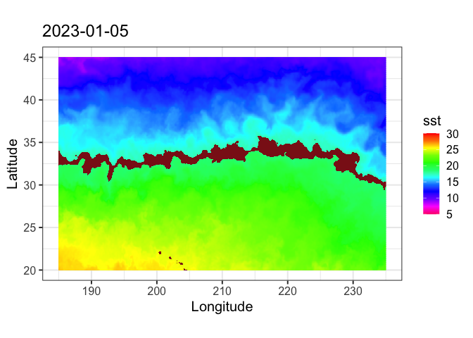
plotBBox(SST, plotColor = 'thermal')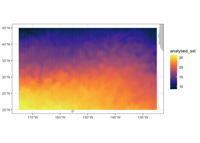
#,maxpixels=1000000)Define and plot the TurtleWatch temperature band
Set the temperature band to 17.5-18.5 degrees C, as determined by the TurtleWatch program.
## Define turtle temperature range
min.temp <- 17.5
max.temp <- 18.5
Create another variable for habitat temperature
Set the habitat temperature to equal NA
SST2 <- SST
SST2$analysed_sst[SST2$analysed_sst >= min.temp & SST2$analysed_sst <= max.temp] <- NA
plotBBox(SST2, plotColor = 'thermal')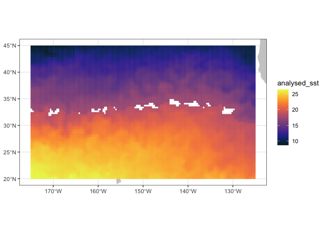
It would be nicer to color in the TurtleWatch band (the NA values) with a different color. If you want to customize graphs, it’s better to use ggplot than the plotBBox that comes with the rerrdapXtracto package. Here we will use ggplot to plot the data. But first the data is reformatted for use in ggplot.
Restructure the data
dims <- dim(SST2$analysed_sst)
SST2.lf <- expand.grid(x=SST$longitude,y=SST$latitude)
SST2.lf$sst<-array(SST2$analysed_sst,dims[1]*dims[2])
Plot the Data using ‘ggplot’
coast <- map_data("worldHires", ylim = ylim, xlim = xlim)

par(mar=c(3,3,.5,.5), las=1, font.axis=10)

myplot<-ggplot(data = SST2.lf, aes(x = x, y = y, fill = sst)) +
  geom_tile(na.rm=T) +
  geom_polygon(data = coast, aes(x=long, y = lat, group = group), fill = "grey80") +
  theme_bw(base_size = 15) + ylab("Latitude") + xlab("Longitude") +
  coord_fixed(1.3,xlim = xlim, ylim = ylim) +
  ggtitle(unique(as.Date(SST2$time))) +
  scale_fill_gradientn(colours = rev(rainbow(12)),limits=c(5,30),na.value = "firebrick4")

myplot