Matching Satellite and Buoy Data
In this exercise, you will combine satellite and buoy data by extracting satellite measurements around specific points defined by buoy locations and dates.
- The focus of this exercise is on matching two data sources from different projections.
- Similar tutorials for mid to lower latitudes can be found at https://github.com/coastwatch-training/CoastWatch-Tutorials.
This exercise demonstrates the following techniques:
- Using ERDDAP to retrieve buoy data in CSV format and satellite data in netCDF format
- Importing and manipulating data with the pandas and xarray libraries
- Resampling data to lower-resolution time steps
- Converting latitude and longitude coordinates to the polar stereographic projection
Data used in this exercise
Ice Surface Temperature, NOAA-20 VIIRS, Near Real-Time, Polar Stereographic (North), 4-day
This dataset provides VIIRS sea ice surface temperature for the Arctic at a 750m resolution, collected by the NOAA-20 satellite. It includes near-real-time daily data and 4-day composites for the past three weeks. For this exercise, we will use 4-day composites data. This dataset is in a polar stereographic projection.
International Arctic Buoy Programme (IABP) Buoy Data, Daily
This dataset is from the US International Arctic Buoy Programme and includes meteorological and oceanographic data from buoys. Dataset is updated daily and includes multiple variables. For this exercise, we will extract surface temperature data.
Satellite Ice Surface Temperature (IST) is measured by the Visible Infrared Imaging Radiometer Suite (VIIRS) and captures the temperature of the surface layer of ice.
Buoy Surface Temperature (Ts) is measured from the bottom of the buoy hull. If the buoy is floating, the reported temperature is of the sea surface. If the buoy is frozen into the ice or sitting on top of it, the reported temperature is of the ground or ice. The freezing temperature of seawater is about -1.8°C, so temperature readings below this indicate ground or ice temperatures.
More details can be found in the metadata section of the data products (click on the data links above).
Load packages
pkgTest <- function(x)
{
  if (!require(x,character.only = TRUE))
  {
    install.packages(x,dep=TRUE)
    if(!require(x,character.only = TRUE)) stop("Package not found")
  }
}

list.of.packages <- c( "ncdf4", "rerddap", "plotdap", "httr",
                       "lubridate", "gridGraphics",  "mapdata",
                       "ggplot2", "RColorBrewer", "grid", "PBSmapping",
                       "rerddapXtracto","dplyr","viridis","cmocean", "sf")

# create list of installed packages
pkges = installed.packages()[,"Package"]

for (pk in list.of.packages) {
  pkgTest(pk)
}
Load buoy data (IABP) from PolarWatch ERDDAP data server
First view information about the data
Use the info function from the rerddap package. The variable surface_temp will be used for this exercise.
ERDDAP_Node = "https://polarwatch.noaa.gov/erddap"

NDBC_id = 'iabpv2_buoys'
NDBC_info=info(datasetid = NDBC_id,url = ERDDAP_Node)

print(NDBC_info)
## <ERDDAP info> iabpv2_buoys
## Base URL: https://polarwatch.noaa.gov/erddap
## Dataset Type: tabledap
## Variables:
## air_temp:
## Range: -90.0, 44.78
## Units: degree_C
## bp:
## Range: 850.0, 1185.9
## Units: mBars
## buoy_id:
## buoy_owner:
## buoy_type:
## day_of_year:
## Range: 6.0E-4, 366.999
## has_air_temp:
## has_bp:
## has_surface_temp:
## hemisphere:
## hour:
## Range: 0.0, 24.0
## latitude:
## Range: -90.0, 90.0
## Units: degrees_north
## logistics:
## longitude:
## Range: -180.0, 180.0
## Units: degrees_east
## minute:
## Range: 0.0, 59.0
## surface_temp:
## Range: -72.88, 45.0
## Units: degree_C
## time:
## Range: 1.189717571E9, 1.729396802E9
## Units: seconds since 1970-01-01T00:00:00Z
## year:
## Range: 2007.0, 2024.0Load the data and put into a data frame
buoy <- rerddap::tabledap(url = ERDDAP_Node, NDBC_id,
                           fields=c('buoy_id', 'latitude',  'longitude', 'time', 'surface_temp',
                           'has_surface_temp'), 'time>=2023-08-01',   'time<=2023-09-30'
)

# Create data frame with the downloaded data
buoy.df <-data.frame(buoy_id=as.character(buoy$buoy_id),
                     longitude=as.numeric(buoy$longitude),
                     latitude=as.numeric(buoy$latitude),
                     time=as.POSIXct(buoy$time, "%Y-%m-%dT%H:%M:%S", tz="UTC"),
                     surface_temp=as.numeric(buoy$surface_temp))

summary(buoy.df)
## buoy_id longitude latitude
## Length:471572 Min. :-180.00 Min. :-74.00
## Class :character 1st Qu.:-129.15 1st Qu.: 73.93
## Mode :character Median : -25.04 Median : 82.74
## Mean : -21.90 Mean : 72.16
## 3rd Qu.: 97.57 3rd Qu.: 85.20
## Max. : 180.00 Max. : 90.00
##
## time surface_temp
## Min. :2023-08-01 00:00:00.00 Min. :-60.00
## 1st Qu.:2023-08-21 16:00:02.00 1st Qu.: -0.95
## Median :2023-09-06 15:00:00.00 Median : 0.30
## Mean :2023-09-04 05:39:11.03 Mean : 1.96
## 3rd Qu.:2023-09-18 17:00:23.00 3rd Qu.: 2.69
## Max. :2023-09-30 00:00:00.00 Max. : 40.00
## NA's :144689head(buoy.df)## buoy_id longitude latitude time surface_temp
## 1 300234066034140 -28.5226 55.0168 2023-08-01 00:00:00 13.5
## 2 300234066034140 -28.5226 55.0168 2023-08-01 01:00:02 13.4
## 3 300234066034140 -28.5226 55.0168 2023-08-01 01:59:57 13.4
## 4 300234066034140 -28.5618 55.0032 2023-08-01 03:00:00 13.4
## 5 300234066034140 -28.5618 55.0032 2023-08-01 04:00:02 13.3
## 6 300234066034140 -28.5618 55.0032 2023-08-01 04:59:57 13.3Select one buoy and process data
We will first select one buoy (buoy id = “300534062897730”). The buoy records measurements at intervals of minutes, resulting in a high-resolution dataset. To align it with the daily resolution of the satellite dataset, we will downsample the buoy data.
Load the data for the target buoy
Check the number of timesteps
# Select one buoy (buoy id = "300534062897730")
target.buoy <- buoy.df %>% filter(buoy_id == "300534062897730")

# Print the number of timestamps before resampling
# cat("# of timesteps before =", nrow(target.buoy), "\n")
#print(c("# of timesteps before =", nrow(target.buoy.daily)))
steps_before <- length(buoy.df$time)

# Resample to daily mean by averaging surface_temp values for each day
# And rename surface_temp to temp_buoy
target.buoy.daily <- target.buoy %>%
  mutate(time = as.Date(time)) %>%
  group_by(time) %>%
  summarize(
    buoy_id = first(buoy_id),
    longitude = first(longitude),
    latitude = first(latitude),
    temp_buoy = mean(surface_temp, na.rm = TRUE))

# Print the number of timesteps after resampling
# cat("# of timesteps before =", nrow(target.buoy.daily), "\n")
steps_after <- length(target.buoy.daily$time)


head(target.buoy.daily)
## # A tibble: 6 × 5
## time buoy_id longitude latitude temp_buoy
## <date> <chr> <dbl> <dbl> <dbl>
## 1 2023-08-01 300534062897730 -144. 86.4 2.19
## 2 2023-08-02 300534062897730 -144. 86.4 1.52
## 3 2023-08-03 300534062897730 -142. 86.3 0.803
## 4 2023-08-04 300534062897730 -142. 86.3 0.542
## 5 2023-08-05 300534062897730 -142. 86.4 0.475
## 6 2023-08-06 300534062897730 -142. 86.5 0.522Verify the reduced number of timesteps
cat("# of timesteps before =", steps_before, "# of timesteps after =", steps_after)## # of timesteps before = 471572 # of timesteps after = 60#length(buoy.df$time)Transform buoy coordinates to polar projection
The buoy locations are provided in latitude and longitude coordinates, whereas the satellite data are in a polar stereographic projection with locations in units of meters. We will convert the buoy locations from latitude and longitude to the corresponding columns and rows in the polar projection.
# Define the projection using the PROJ4 string format
proj4text <- "+proj=stere +lat_0=90 +lat_ts=70 +lon_0=-45 +k=1 +x_0=0 +y_0=0 +datum=WGS84 +units=m +no_defs"

# Convert the dataframe into an sf object (Spatial Dataframe)
target.buoy.sf <- st_as_sf(target.buoy.daily, coords = c("longitude", "latitude"), crs = 4326)

# Reproject the data to the Polar Stereographic projection using the PROJ4 string
target.buoy.projected <- st_transform(target.buoy.sf, crs = proj4text)

# Extract the projected coordinates
target.buoy.projected$cols <- st_coordinates(target.buoy.projected)[,1] # X (columns)
target.buoy.projected$rows <- st_coordinates(target.buoy.projected)[,2] # Y (rows)

# Show the first 2 rows to verify that the 'cols' and 'rows' columns were added
head(target.buoy.projected, 2)
## Simple feature collection with 2 features and 5 fields
## Geometry type: POINT
## Dimension: XY
## Bounding box: xmin: -389549.6 ymin: 58944.53 xmax: -385824.4 ymax: 59121.58
## Projected CRS: +proj=stere +lat_0=90 +lat_ts=70 +lon_0=-45 +k=1 +x_0=0 +y_0=0 +datum=WGS84 +units=m +no_defs
## # A tibble: 2 × 6
## time buoy_id temp_buoy geometry cols rows
## <date> <chr> <dbl> <POINT [m]> <dbl> <dbl>
## 1 2023-08-01 300534062897730 2.19 (-385824.4 58944.53) -385824. 58945.
## 2 2023-08-02 300534062897730 1.52 (-389549.6 59121.58) -389550. 59122.# Select the first buoy location to pull corresponding satellite data
target.buoy.cols <- target.buoy.projected$cols[1]
target.buoy.rows <- target.buoy.projected$rows[1]
# Verify the data
print(target.buoy.cols)## [1] -385824.4print(target.buoy.rows)## [1] 58944.53Load satellite data from PolarWatch
Look at the metadata to check the metadata Note that the temperature is in degrees Kelvin.
NDBC_id_2 = 'noaacwVIIRSn20icesrftempNP06Daily4Day'
NDBC_info_2=info(datasetid = NDBC_id_2,url = ERDDAP_Node)

print(NDBC_info_2)
## <ERDDAP info> noaacwVIIRSn20icesrftempNP06Daily4Day
## Base URL: https://polarwatch.noaa.gov/erddap
## Dataset Type: griddap
## Dimensions (range):
## time: (2021-04-13T00:00:00Z, 2024-10-15T00:00:00Z)
## altitude: (0.0, 0.0)
## rows: (-3434002.5, 3434002.5)
## cols: (-3434002.5, 3434002.5)
## Variables:
## IceSrfTemp:
## Units: Kelvin(K)Extract the satellite ice surface temperture timeseries
Use the rxtracto function from the rerddapXtracto package
zpos <- rep(0., length(target.buoy.projected$time))

sat_data <- rxtracto(NDBC_info_2,
                    xName="cols",
                    yName="rows",
                    tName="time",
                    zName="altitude",
                    parameter="IceSrfTemp",
                    xcoord = target.buoy.projected$cols,
                    ycoord = target.buoy.projected$rows,
                    tcoord = target.buoy.projected$time,
                    zcoord = zpos
                    )
head(sat_data)
## $`mean IceSrfTemp`
## [1] 272.9286 NaN NaN NaN NaN NaN 271.0790 270.2815
## [9] NaN NaN NaN 272.5218 NaN 271.7425 272.3054 270.4868
## [17] 270.3914 273.3692 273.4933 272.3756 273.1550 273.1486 273.4222 NaN
## [25] NaN NaN NaN 269.4200 268.0554 267.6486 268.2197 NaN
## [33] NaN NaN NaN NaN 266.4402 268.3176 268.0433 267.8826
## [41] 268.3053 NaN NaN NaN NaN NaN NaN 270.8179
## [49] NaN NaN NaN NaN 264.4946 263.8606 NaN NaN
## [57] 256.9289 NaN NaN NaN
##
## $`stdev IceSrfTemp`
## [1] NA NA NA NA NA NA NA NA NA NA NA NA NA NA NA NA NA NA NA NA NA NA NA NA NA
## [26] NA NA NA NA NA NA NA NA NA NA NA NA NA NA NA NA NA NA NA NA NA NA NA NA NA
## [51] NA NA NA NA NA NA NA NA NA NA
##
## $n
## [1] 1 0 0 0 0 0 1 1 0 0 0 1 0 1 1 1 1 1 1 1 1 1 1 0 0 0 0 1 1 1 1 0 0 0 0 0 1 1
## [39] 1 1 1 0 0 0 0 0 0 1 0 0 0 0 1 1 0 0 1 0 0 0
##
## $`satellite date`
## [1] "2023-08-01T00:00:00Z" "2023-08-02T00:00:00Z" "2023-08-03T00:00:00Z"
## [4] "2023-08-04T00:00:00Z" "2023-08-05T00:00:00Z" "2023-08-06T00:00:00Z"
## [7] "2023-08-07T00:00:00Z" "2023-08-08T00:00:00Z" "2023-08-09T00:00:00Z"
## [10] "2023-08-10T00:00:00Z" "2023-08-11T00:00:00Z" "2023-08-12T00:00:00Z"
## [13] "2023-08-13T00:00:00Z" "2023-08-14T00:00:00Z" "2023-08-15T00:00:00Z"
## [16] "2023-08-16T00:00:00Z" "2023-08-17T00:00:00Z" "2023-08-18T00:00:00Z"
## [19] "2023-08-19T00:00:00Z" "2023-08-20T00:00:00Z" "2023-08-21T00:00:00Z"
## [22] "2023-08-22T00:00:00Z" "2023-08-23T00:00:00Z" "2023-08-24T00:00:00Z"
## [25] "2023-08-25T00:00:00Z" "2023-08-26T00:00:00Z" "2023-08-27T00:00:00Z"
## [28] "2023-08-28T00:00:00Z" "2023-08-29T00:00:00Z" "2023-08-30T00:00:00Z"
## [31] "2023-08-31T00:00:00Z" "2023-09-01T00:00:00Z" "2023-09-02T00:00:00Z"
## [34] "2023-09-03T00:00:00Z" "2023-09-04T00:00:00Z" "2023-09-05T00:00:00Z"
## [37] "2023-09-06T00:00:00Z" "2023-09-07T00:00:00Z" "2023-09-08T00:00:00Z"
## [40] "2023-09-09T00:00:00Z" "2023-09-10T00:00:00Z" "2023-09-11T00:00:00Z"
## [43] "2023-09-12T00:00:00Z" "2023-09-13T00:00:00Z" "2023-09-14T00:00:00Z"
## [46] "2023-09-15T00:00:00Z" "2023-09-16T00:00:00Z" "2023-09-17T00:00:00Z"
## [49] "2023-09-18T00:00:00Z" "2023-09-19T00:00:00Z" "2023-09-20T00:00:00Z"
## [52] "2023-09-21T00:00:00Z" "2023-09-22T00:00:00Z" "2023-09-23T00:00:00Z"
## [55] "2023-09-24T00:00:00Z" "2023-09-25T00:00:00Z" "2023-09-26T00:00:00Z"
## [58] "2023-09-27T00:00:00Z" "2023-09-28T00:00:00Z" "2023-09-29T00:00:00Z"
##
## $`requested x min`
## [1] -385824.4 -389549.6 -398253.9 -399928.2 -383575.3 -376519.9 -373178.9
## [8] -369485.9 -364101.8 -358053.1 -344667.3 -339413.6 -325379.7 -308859.0
## [15] -297005.5 -290218.6 -283776.4 -280170.8 -271276.3 -263223.8 -263830.1
## [22] -269754.9 -268728.9 -262726.0 -258730.5 -262527.7 -277050.1 -274674.6
## [29] -261436.0 -250715.5 -248618.1 -253833.2 -247254.1 -241801.9 -248913.6
## [36] -253308.9 -253242.1 -259535.5 -256109.5 -263955.3 -260399.8 -254873.5
## [43] -244906.9 -239308.2 -230283.9 -227856.9 -220466.8 -213128.6 -205585.0
## [50] -194830.9 -185590.9 -183007.2 -178188.9 -176271.0 -179406.9 -180725.3
## [57] -176656.0 -171027.2 -162577.7 -149611.3
##
## $`requested x max`
## [1] -385824.4 -389549.6 -398253.9 -399928.2 -383575.3 -376519.9 -373178.9
## [8] -369485.9 -364101.8 -358053.1 -344667.3 -339413.6 -325379.7 -308859.0
## [15] -297005.5 -290218.6 -283776.4 -280170.8 -271276.3 -263223.8 -263830.1
## [22] -269754.9 -268728.9 -262726.0 -258730.5 -262527.7 -277050.1 -274674.6
## [29] -261436.0 -250715.5 -248618.1 -253833.2 -247254.1 -241801.9 -248913.6
## [36] -253308.9 -253242.1 -259535.5 -256109.5 -263955.3 -260399.8 -254873.5
## [43] -244906.9 -239308.2 -230283.9 -227856.9 -220466.8 -213128.6 -205585.0
## [50] -194830.9 -185590.9 -183007.2 -178188.9 -176271.0 -179406.9 -180725.3
## [57] -176656.0 -171027.2 -162577.7 -149611.3Convert degrees K to degrees C
#sftemp_ds_subset$temp_sat <- sftemp_ds_subset$IceSrfTemp - 273.15
temp_sat <- sat_data$mean - 273.15
temp_sat
## [1] -0.221441650 NaN NaN NaN NaN
## [6] NaN -2.070959473 -2.868536377 NaN NaN
## [11] NaN -0.628179932 NaN -1.407537842 -0.844641113
## [16] -2.663214111 -2.758581543 0.219171143 0.343347168 -0.774359131
## [21] 0.004998779 -0.001409912 0.272210693 NaN NaN
## [26] NaN NaN -3.729956055 -5.094610596 -5.501409912
## [31] -4.930303955 NaN NaN NaN NaN
## [36] NaN -6.709814453 -4.832434082 -5.106665039 -5.267431641
## [41] -4.844671631 NaN NaN NaN NaN
## [46] NaN NaN -2.332067871 NaN NaN
## [51] NaN NaN -8.655371094 -9.289373779 NaN
## [56] NaN -16.221136475 NaN NaN NaN#extract$meanMerge Buoy and Satellite Data
Add the satellite ice temperature to the buoy dataset. Not all buoy dates have corresponding satellite data. Any unmatched dates will be filled with NaN values.
target.buoy.projected$temp_sat <- temp_sat
head(target.buoy.projected)
## Simple feature collection with 6 features and 6 fields
## Geometry type: POINT
## Dimension: XY
## Bounding box: xmin: -399928.2 ymin: 46312.22 xmax: -376519.9 ymax: 59121.58
## Projected CRS: +proj=stere +lat_0=90 +lat_ts=70 +lon_0=-45 +k=1 +x_0=0 +y_0=0 +datum=WGS84 +units=m +no_defs
## # A tibble: 6 × 7
## time buoy_id temp_buoy geometry cols rows temp_sat
## <date> <chr> <dbl> <POINT [m]> <dbl> <dbl> <dbl>
## 1 2023-08-01 300534… 2.19 (-385824.4 58944.53) -385824. 58945. -0.221
## 2 2023-08-02 300534… 1.52 (-389549.6 59121.58) -389550. 59122. NaN
## 3 2023-08-03 300534… 0.803 (-398253.9 50891.54) -398254. 50892. NaN
## 4 2023-08-04 300534… 0.542 (-399928.2 48358.67) -399928. 48359. NaN
## 5 2023-08-05 300534… 0.475 (-383575.3 49983.71) -383575. 49984. NaN
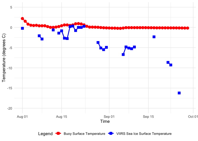
## 6 2023-08-06 300534… 0.522 (-376519.9 46312.22) -376520. 46312. NaNVisualize Matched DataSets
Visualize the matched buoy and satellite datasets to assess the data alignment.
# Create the plot
ggplot(target.buoy.projected, aes(x = time)) +
  # Plot the buoy data
  geom_point(aes(y = temp_buoy, color = 'Buoy Surface Temperature'), size =3) +
  geom_line(aes(y = temp_buoy, color = 'Buoy Surface Temperature'), linewidth = 1, na.rm = TRUE) +

  # Plot the satellite (VIIRS Sea Ice Surface Temperature) data
  geom_point(aes(y = temp_sat, color = 'VIIRS Sea Ice Surface Temperature'), shape = 15, size = 3) +
  geom_line(aes(y = temp_sat, color = 'VIIRS Sea Ice Surface Temperature'), linewidth = 1, na.rm = TRUE) +

  # Set the y-axis limits
  ylim(-20, 5) +

  # Labels and theme
  labs(x = 'Time', y = 'Temperature (degrees C)', color = 'Legend') +
  scale_color_manual(values = c('Buoy Surface Temperature' = 'red',
                                'VIIRS Sea Ice Surface Temperature' = 'blue')) +
  theme_minimal() +
  theme(legend.position = "bottom")