Extract data within a boundary

History | Updated Sep 2023

Background

One use for satellite observations is to supplement in situ sampling of geographical locations where the timespan or frequency measurements, or spatial dimensions or remoteness of the locations, make physical sampling impossible or impractical. One drawback is that satellite data are often rectangular, whereas geographical locations can have irregular boundaries. Examples of locations with boundaries include Marine Protected Areas or marine physical, biological, and ecological divisions like the Longhurst Marine Provinces.

Objectives

In this tutorial we will learn how to download a timeseries of SST satellite data from an ERDDAP server, and then mask the data to retain only the data within an irregular geographical boundary (polygon). We will then plot a yearly seasonal cycle from within the boundary.

The tutorial demonstrates the following techniques

• Downloading data from an ERDDAP data server
• Visualizing data on a map
• Masking satellite data using a shape file

Datasets used

NOAA Geo-polar Blended Analysis Sea-Surface Temperature, Global, Monthly, 5km, 2019-Present
The NOAA geo-polar blended SST is a high resolution satellite-based sea surface temperature (SST) product that combines SST data from US, Japanese and European geostationary infrared imagers, and low-earth orbiting infrared (U.S. and European) SST data, into a single product. We will use the monthly composite. https://coastwatch.pfeg.noaa.gov/erddap/griddap/NOAA_DHW_monthly

Longhurst Marine Provinces
The dataset represents the division of the world oceans into provinces as defined by Longhurst (1995; 1998; 2006). This division has been based on the prevailing role of physical forcing as a regulator of phytoplankton distribution. The Longhurst Marine Provinces dataset is available online (https://www.marineregions.org/downloads.php) and within the shapes folder associated with this repository. For this tutorial we will use the Gulf Stream province (ProvCode: GFST)

../images/longhurst.png

Import packages

Note: Make sure you have at least version 0.10.0 of regionmask * To install with conda use “conda install -c conda-forge regionmask=0.10.0 cartopy”

import matplotlib.pyplot as plt
import xarray as xr
import geopandas
import regionmask
import cartopy.crs as ccrs
import cartopy.feature as cfeature
from cartopy.mpl.ticker import LongitudeFormatter, LatitudeFormatter
import warnings
import os
warnings.filterwarnings('ignore')

Load the Longhurst Provinces shape files into a geopandas dataframe

#shape_path = '../resources/longhurst_v4_2010/Longhurst_world_v4_2010.shp'
shape_path = os.path.join('..',
                          'resources',
                          'longhurst_v4_2010',
                          'Longhurst_world_v4_2010.shp'
                          )
shapefiles = geopandas.read_file(shape_path)
shapefiles.head(8)

	ProvCode	ProvDescr	geometry
0	BPLR	Polar - Boreal Polar Province (POLR)	MULTIPOLYGON (((-161.18426 63.50000, -161.5000...
1	ARCT	Polar - Atlantic Arctic Province	MULTIPOLYGON (((-21.51305 64.64409, -21.55945 ...
2	SARC	Polar - Atlantic Subarctic Province	MULTIPOLYGON (((11.26472 63.96082, 11.09548 63...
3	NADR	Westerlies - N. Atlantic Drift Province (WWDR)	POLYGON ((-11.50000 57.50000, -11.50000 56.500...
4	GFST	Westerlies - Gulf Stream Province	POLYGON ((-43.50000 43.50000, -43.50000 42.500...
5	NASW	Westerlies - N. Atlantic Subtropical Gyral Pro...	POLYGON ((-39.50000 25.50000, -40.50000 25.500...
6	NATR	Trades - N. Atlantic Tropical Gyral Province (...	MULTIPOLYGON (((-72.34673 18.53597, -72.36877 ...
7	WTRA	Trades - Western Tropical Atlantic Province	POLYGON ((-19.50000 -6.50000, -20.50000 -6.500...

Isolate the Gulf Stream Province

The Gulf Stream Province can be isolated using its ProvCode (GFST)

ProvCode = "GFST"

# Locate the row with the ProvCode code
gulf_stream = shapefiles.loc[shapefiles["ProvCode"] == ProvCode]
gulf_stream

	ProvCode	ProvDescr	geometry
4	GFST	Westerlies - Gulf Stream Province	POLYGON ((-43.50000 43.50000, -43.50000 42.500...

Find the coordinates of the bounding box

• The bounding box is the smallest rectangle that will completely enclose the province.
• We will use the bounding box coordinates to subset the satellite data

gs_bnds = gulf_stream.bounds
gs_bnds

	minx	miny	maxx	maxy
4	-73.5	33.5	-43.5	43.5

Open the satellite dataset into a xarray dataset object

erddap_url = '/'.join(['https://coastwatch.pfeg.noaa.gov',
                       'erddap',
                       'griddap',
                       'NOAA_DHW_monthly'
                       ])

ds = xr.open_dataset(erddap_url)
ds

<xarray.Dataset>
Dimensions:                          (time: 464, latitude: 3600, longitude: 7200)
Coordinates:
  * time                             (time) datetime64[ns] 1985-01-16 ... 202...
  * latitude                         (latitude) float32 89.97 89.93 ... -89.97
  * longitude                        (longitude) float32 -180.0 -179.9 ... 180.0
Data variables:
    sea_surface_temperature          (time, latitude, longitude) float32 ...
    mask                             (time, latitude, longitude) float32 ...
    sea_surface_temperature_anomaly  (time, latitude, longitude) float32 ...
Attributes: (12/66)
    _NCProperties:                    version=2,netcdf=4.8.1,hdf5=1.12.2
    acknowledgement:                  NOAA Coral Reef Watch program
    cdm_data_type:                    Grid
    comment:                          This is a product of NOAA Coral Reef Wa...
    contributor_name:                 NOAA Coral Reef Watch program
    contributor_role:                 Collecting source data and deriving pro...
    ...                               ...
    time_coverage_duration:           P1M
    time_coverage_end:                2023-08-16T00:00:00Z
    time_coverage_resolution:         P1M
    time_coverage_start:              1985-01-16T00:00:00Z
    title:                            SST and SST Anomaly, NOAA Global Coral ...
    Westernmost_Easting:              -179.975

xarray.Dataset

• Dimensions:
  • time: 464
  • latitude: 3600
  • longitude: 7200
• Coordinates: (3)
  • time
    (time)
    datetime64[ns]
    1985-01-16 ... 2023-08-16

    _CoordinateAxisType :

    Time

    actual_range :

    [4.746816e+08 1.692144e+09]

    axis :

    T

    coverage_content_type :

    coordinate

    ioos_category :

    Time

    long_name :

    reference time of the last day of the composite temporal coverage

    standard_name :

    time

    time_origin :

    01-JAN-1970 00:00:00

    array(['1985-01-16T00:00:00.000000000', '1985-02-16T00:00:00.000000000',
           '1985-03-16T00:00:00.000000000', ..., '2023-06-16T00:00:00.000000000',
           '2023-07-16T00:00:00.000000000', '2023-08-16T00:00:00.000000000'],
          dtype='datetime64[ns]')

  • latitude
    (latitude)
    float32
    89.97 89.93 89.88 ... -89.92 -89.97

    _CoordinateAxisType :

    Lat

    actual_range :

    [-89.975 89.975]

    axis :

    Y

    comment :

    equirectangular projection and grid centers

    coverage_content_type :

    coordinate

    ioos_category :

    Location

    long_name :

    Latitude

    standard_name :

    latitude

    units :

    degrees_north

    valid_max :

    89.975

    valid_min :

    -89.975

    array([ 89.975   ,  89.92501 ,  89.87501 , ..., -89.875   , -89.924995,
           -89.975   ], dtype=float32)

  • longitude
    (longitude)
    float32
    -180.0 -179.9 ... 179.9 180.0

    _CoordinateAxisType :

    Lon

    actual_range :

    [-179.975 179.975]

    axis :

    X

    comment :

    equirectangular projection and grid centers

    coverage_content_type :

    coordinate

    ioos_category :

    Location

    long_name :

    Longitude

    standard_name :

    longitude

    units :

    degrees_east

    valid_max :

    179.975

    valid_min :

    -179.975

    array([-179.975  , -179.925  , -179.875  , ...,  179.875  ,  179.92499,
            179.975  ], dtype=float32)

• Data variables: (3)
  • sea_surface_temperature
    (time, latitude, longitude)
    float32
    ...

    colorBarMaximum :

    32.0

    colorBarMinimum :

    0.0

    coverage_content_type :

    physicalMeasurement

    ioos_category :

    Temperature

    long_name :

    analysed sea surface temperature

    standard_name :

    sea_surface_temperature

    units :

    degree_C

    valid_max :

    50.0

    valid_min :

    -2.0

    [12026880000 values with dtype=float32]

  • mask
    (time, latitude, longitude)
    float32
    ...

    colorBarMaximum :

    5.0

    colorBarMinimum :

    0.0

    comment :

    A 2D array, in the same size as the data array in the X and Y directions, the classifies land, ice pixels, and water (data) pixels

    coverage_content_type :

    thematicClassification

    flag_meanings :

    valid-water land missing ice

    flag_values :

    [0 1 2 4]

    ioos_category :

    Quality

    long_name :

    Pixel characteristics flag array

    units :

    pixel_classification

    [12026880000 values with dtype=float32]

  • sea_surface_temperature_anomaly
    (time, latitude, longitude)
    float32
    ...

    colorBarMaximum :

    3.0

    colorBarMinimum :

    -3.0

    coverage_content_type :

    physicalMeasurement

    ioos_category :

    Temperature

    long_name :

    sea surface temperature anomaly

    standard_name :

    surface_temperature_anomaly

    units :

    degree_C

    valid_max :

    15.0

    valid_min :

    -15.0

    [12026880000 values with dtype=float32]

• Indexes: (3)
  • time
    PandasIndex

    PandasIndex(DatetimeIndex(['1985-01-16 00:00:00', '1985-02-16 00:00:00',
                   '1985-03-16 00:00:00', '1985-04-16 00:00:00',
                   '1985-05-15 23:00:00', '1985-06-15 23:00:00',
                   '1985-07-15 23:00:00', '1985-08-15 23:00:00',
                   '1985-09-15 23:00:00', '1985-10-15 23:00:00',
                   ...
                   '2022-11-16 00:00:00', '2022-12-16 00:00:00',
                   '2023-01-16 00:00:00', '2023-02-16 00:00:00',
                   '2023-03-16 00:00:00', '2023-04-16 00:00:00',
                   '2023-05-16 00:00:00', '2023-06-16 00:00:00',
                   '2023-07-16 00:00:00', '2023-08-16 00:00:00'],
                  dtype='datetime64[ns]', name='time', length=464, freq=None))

  • latitude
    PandasIndex

    PandasIndex(Index([  89.9749984741211,  89.92501068115234,  89.87500762939453,
            89.82500457763672,   89.7750015258789,   89.7249984741211,
            89.67501068115234,  89.62500762939453,  89.57500457763672,
             89.5250015258789,
           ...
            -89.5250015258789, -89.57499694824219,            -89.625,
           -89.67499542236328,  -89.7249984741211,  -89.7750015258789,
           -89.82499694824219,            -89.875, -89.92499542236328,
            -89.9749984741211],
          dtype='float32', name='latitude', length=3600))

  • longitude
    PandasIndex

    PandasIndex(Index([-179.97500610351562,  -179.9250030517578,            -179.875,
           -179.82501220703125, -179.77500915527344, -179.72500610351562,
            -179.6750030517578,            -179.625, -179.57501220703125,
           -179.52500915527344,
           ...
            179.52499389648438,  179.57501220703125,             179.625,
            179.67498779296875,  179.72500610351562,  179.77499389648438,
            179.82501220703125,             179.875,  179.92498779296875,
            179.97500610351562],
          dtype='float32', name='longitude', length=7200))

• Attributes: (66)

  _NCProperties :

  version=2,netcdf=4.8.1,hdf5=1.12.2

  acknowledgement :

  NOAA Coral Reef Watch program

  cdm_data_type :

  Grid

  comment :

  This is a product of NOAA Coral Reef Watch Global 5km Satellite Coral Bleaching Heat Stress Monitoring Product Suite Version 3.1, derived from CoralTemp v1.0.

  contributor_name :

  NOAA Coral Reef Watch program

  contributor_role :

  Collecting source data and deriving products; performing quality control of products; disseminating, storing, and submitting data to archive.

  Conventions :

  CF-1.6, ACDD-1.3, COARDS

  creator_email :

  coralreefwatch@noaa.gov

  creator_institution :

  NOAA/NESDIS/STAR Coral Reef Watch program

  creator_name :

  NOAA Coral Reef Watch program

  creator_type :

  group

  creator_url :

  https://coralreefwatch.noaa.gov

  date_created :

  2018-03-01T12:00:00Z

  date_issued :

  2019-01-19T20:32:23Z

  date_metadata_modified :

  2018-09-01T12:00:00Z

  date_modified :

  2018-03-01T12:00:00Z

  Easternmost_Easting :

  179.975

  geospatial_bounds :

  POLYGON((-90.0 180.0, 90.0 180.0, 90.0 -180.0, -90.0 -180.0, -90.0 180.0))

  geospatial_bounds_crs :

  EPSG:4326

  geospatial_lat_max :

  89.975

  geospatial_lat_min :

  -89.975

  geospatial_lat_units :

  degrees_north

  geospatial_lon_max :

  179.975

  geospatial_lon_min :

  -179.975

  geospatial_lon_units :

  degrees_east

  grid_mapping_epsg_code :

  EPSG:32663

  grid_mapping_inverse_flattening :

  298.2572

  grid_mapping_name :

  latitude_longitude

  grid_mapping_semi_major_axis :

  6378137.0

  history :

  Tue Jul 27 10:37:54 2021: ncrename -d lon,longitude -d lat,latitude -v lon,longitude -v lat,latitude -v sea surface temperature anomaly,sea_surface_temperature_anomaly /cwdata/coralreef/work/temp.nc Monthly data files for mean sea surface temperature (SST) and sea surface temperature anomaly (SST anomaly) were downloaded from ftp.star.nesdis.noaa.gov/pub/sod/mecb/crw/data/5km/v3.1/nc/v1.0/monthly. Monthly files were created that contain both SST and SST anomaly data, and a mask of earth surface classifications. 2023-09-06T18:39:14Z (local files) 2023-09-06T18:39:14Z http://coastwatch.pfeg.noaa.gov/erddap/griddap/NOAA_DHW_monthly.das

  id :

  Satellite_Global_5km_CoralTemp_SST_SSTA_Monthly_Mean_Composite

  infoUrl :

  https://coralreefwatch.noaa.gov/product/5km/index.php

  institution :

  NOAA/NESDIS/STAR Coral Reef Watch program

  instrument :

  ATSR-1, ATSR-2, AATSR, AVHRR, AVHRR-2, AVHRR-3, VIIRS, GOES Imager, MTSAT Imager, MTSAT 2 Imager, AHI, ABI, SEVIRI, buoy - moored buoy, buoy - drifting buoy, buoy - TAO buoy, surface seawater intake

  instrument_vocabulary :

  NOAA NODC Ocean Archive System Instruments

  keywords :

  5km, analysed, anomaly, array, characteristics, coral, crw, data, earth, Earth Science > Land Surface > Land Temperature > Land Surface Temperature, Earth Science > Oceans > Ocean Temperature > Sea Surface Temperature, Earth Science > Oceans > Ocean Temperature > Sea Surface Temperature Anomaly, Earth Science > Oceans > Ocean Temperature > Water Temperature, Earth Science > Spectral/Engineering > Infrared Wavelengths > Thermal Infrared, engineering, environmental, flag, global, information, infrared, land, latitude, longitude, mask, mean, month, monthly, national, nesdis, noaa, ocean, oceans, pixel, program, quality, reef, satellite, science, sea, sea_surface_temperature, sea_surface_temperature_anomaly, seawater, service, spectral, spectral/engineering, sst, star, surface, surface_temperature_anomaly, temperature, thermal, time, v.3.1, watch, water, wavelengths

  keywords_vocabulary :

  GCMD Science Keywords

  license :

  The data produced by Coral Reef Watch are available for use without restriction, but Coral Reef Watch relies on the ethics and integrity of the user to ensure that the source of the data and products is appropriately cited and credited. When using these data and products, credit and courtesy should be given to NOAA Coral Reef Watch. Please include the appropriate DOI associated with this dataset in the citation. For more information, visit the NOAA Coral Reef Watch website: https://coralreefwatch.noaa.gov. Recommendations for citing and providing credit are provided at https://coralreefwatch.noaa.gov/satellite/docs/recommendations_crw_citation.php. Users are referred to the footer section of the Coral Reef Watch website (https://coralreefwatch.noaa.gov/index.php) for disclaimers, policies, notices pertaining to the use of the data.

  metadata_link :

  https://coralreefwatch.noaa.gov/product/5km/index.php

  naming_authority :

  gov.noaa.coralreefwatch

  NCO :

  "4.6.3"

  Northernmost_Northing :

  89.975

  platform :

  Ships, drifting buoys, moored buoys, TOGA-TAO buoy arrays, GOES-8 satellite, GOES-9 satellite, GOES-10 satellite, GOES-11 satellite, GOES-12 satellite, GOES-13 satellite, GOES-14 satellite, GOES-15 satellite, GOES-16 satellite, MTSAT-1R satellite, MTSAT-2 satellite, Himawari-8 satellite, Meteosat-8 satellite, Meteosat-9 satellite, Meteoset-10 satellite, Meteosat-11 satellite, Suomi NPP, MetOp-A satellite, MetOp-B satellite, NOAA-9 satellite, NOAA-11 satellite, NOAA-12 satellite, NOAA-14 satellite, NOAA-15 satellite, NOAA-16 satellite, NOAA-17 satellite, NOAA-18 satellite, NOAA-19 satellite.

  platform_vocabulary :

  NOAA NODC Ocean Archive System Platforms

  processing_level :

  Derived from L4 satellite sea surface temperature analysis

  product_version :

  3.1

  program :

  NOAA Coral Reef Watch program

  project :

  NOAA Coral Reef Watch program

  publisher_email :

  erd.data at noaa.gov

  publisher_institution :

  NOAA/NESDIS/STAR Coral Reef Watch program

  publisher_name :

  NOAA NMFS SWFSC ERD, CoastWatch West Coast Node

  publisher_type :

  institution

  publisher_url :

  https://coralreefwatch.noaa.gov, https://coastwatch.pfeg.noaa.gov/

  references :

  https://coralreefwatch.noaa.gov/product/5km/index.php and https://coralreefwatch.noaa.gov/satellite/coraltemp.php

  source :

  Coral Reef Watch CoralTemp v1.0

  sourceUrl :

  (local files)

  Southernmost_Northing :

  -89.975

  spatial_resolution :

  0.05 degree

  standard_name_vocabulary :

  CF Standard Name Table v27

  summary :

  This is a product of NOAA Coral Reef Watch Global 5km Satellite Coral Bleaching Heat Stress Monitoring Product Suite, derived from CoralTemp v1.0.

  time_coverage_duration :

  P1M

  time_coverage_end :

  2023-08-16T00:00:00Z

  time_coverage_resolution :

  P1M

  time_coverage_start :

  1985-01-16T00:00:00Z

  title :

  SST and SST Anomaly, NOAA Global Coral Bleaching Monitoring, 5km, V.3.1, Monthly, 1985-Present

  Westernmost_Easting :

  -179.975

Subset the satellite data

• Use the bounding box coordinates for the latitude and longitude slices
• Select the entire year of 2020

# This dataset has latitude in descending order. 
# Therefore use maxy first and miny last to slice latitude
ds_subset = ds['sea_surface_temperature'].sel(time=slice("2020-01-16", "2020-12-16"),
                                              latitude=slice(gs_bnds.maxy.item(), 
                                                             gs_bnds.miny.item()),
                                              longitude=slice(gs_bnds.minx.item(), 
                                                              gs_bnds.maxx.item())
                                            )
ds_subset

<xarray.DataArray 'sea_surface_temperature' (time: 12, latitude: 200,
                                             longitude: 600)>
[1440000 values with dtype=float32]
Coordinates:
  * time       (time) datetime64[ns] 2020-01-16 2020-02-16 ... 2020-12-16
  * latitude   (latitude) float32 43.47 43.43 43.38 43.33 ... 33.62 33.58 33.53
  * longitude  (longitude) float32 -73.47 -73.42 -73.38 ... -43.62 -43.57 -43.53
Attributes:
    colorBarMaximum:        32.0
    colorBarMinimum:        0.0
    coverage_content_type:  physicalMeasurement
    ioos_category:          Temperature
    long_name:              analysed sea surface temperature
    standard_name:          sea_surface_temperature
    units:                  degree_C
    valid_max:              50.0
    valid_min:              -2.0

xarray.DataArray

'sea_surface_temperature'

• time: 12
• latitude: 200
• longitude: 600

• ...

  [1440000 values with dtype=float32]

• Coordinates: (3)
  • time
    (time)
    datetime64[ns]
    2020-01-16 ... 2020-12-16

    _CoordinateAxisType :

    Time

    actual_range :

    [4.746816e+08 1.692144e+09]

    axis :

    T

    coverage_content_type :

    coordinate

    ioos_category :

    Time

    long_name :

    reference time of the last day of the composite temporal coverage

    standard_name :

    time

    time_origin :

    01-JAN-1970 00:00:00

    array(['2020-01-16T00:00:00.000000000', '2020-02-16T00:00:00.000000000',
           '2020-03-15T23:00:00.000000000', '2020-04-15T23:00:00.000000000',
           '2020-05-15T23:00:00.000000000', '2020-06-15T23:00:00.000000000',
           '2020-07-15T23:00:00.000000000', '2020-08-15T23:00:00.000000000',
           '2020-09-15T23:00:00.000000000', '2020-10-15T23:00:00.000000000',
           '2020-11-16T00:00:00.000000000', '2020-12-16T00:00:00.000000000'],
          dtype='datetime64[ns]')

  • latitude
    (latitude)
    float32
    43.47 43.43 43.38 ... 33.58 33.53

    _CoordinateAxisType :

    Lat

    actual_range :

    [-89.975 89.975]

    axis :

    Y

    comment :

    equirectangular projection and grid centers

    coverage_content_type :

    coordinate

    ioos_category :

    Location

    long_name :

    Latitude

    standard_name :

    latitude

    units :

    degrees_north

    valid_max :

    89.975

    valid_min :

    -89.975

    array([43.475   , 43.42501 , 43.375008, 43.325005, 43.275   , 43.225   ,
           43.17501 , 43.125008, 43.075005, 43.025   , 42.975   , 42.92501 ,
           42.875008, 42.825005, 42.775   , 42.725   , 42.67501 , 42.625008,
           42.575005, 42.525   , 42.475   , 42.42501 , 42.375008, 42.325005,
           42.275   , 42.225   , 42.17501 , 42.125008, 42.075005, 42.025   ,
           41.975   , 41.92501 , 41.875008, 41.825005, 41.775   , 41.725   ,
           41.67501 , 41.625008, 41.575005, 41.525   , 41.475   , 41.42501 ,
           41.375008, 41.325005, 41.275   , 41.225   , 41.17501 , 41.125008,
           41.075005, 41.025   , 40.975   , 40.92501 , 40.875008, 40.825005,
           40.775   , 40.725   , 40.67501 , 40.625008, 40.575005, 40.525   ,
           40.475   , 40.42501 , 40.375008, 40.325005, 40.275   , 40.225   ,
           40.17501 , 40.125008, 40.075005, 40.025   , 39.975   , 39.92501 ,
           39.875008, 39.825005, 39.775   , 39.725   , 39.67501 , 39.625008,
           39.575005, 39.525   , 39.475   , 39.42501 , 39.375008, 39.325005,
           39.275   , 39.225   , 39.17501 , 39.125008, 39.075005, 39.025   ,
           38.975   , 38.92501 , 38.875008, 38.825005, 38.775   , 38.725   ,
           38.67501 , 38.625008, 38.575005, 38.525   , 38.475   , 38.42501 ,
           38.375008, 38.325005, 38.275   , 38.225   , 38.17501 , 38.125008,
           38.075005, 38.025   , 37.975006, 37.925003, 37.875   , 37.825005,
           37.775   , 37.725006, 37.675003, 37.625   , 37.575005, 37.525   ,
           37.475006, 37.425003, 37.375   , 37.325005, 37.275   , 37.225006,
           37.175003, 37.125   , 37.075005, 37.025   , 36.975006, 36.925003,
           36.875   , 36.825005, 36.775   , 36.725006, 36.675003, 36.625   ,
           36.575005, 36.525   , 36.475006, 36.425003, 36.375   , 36.325005,
           36.275   , 36.225006, 36.175003, 36.125   , 36.075005, 36.025   ,
           35.975006, 35.925003, 35.875   , 35.825005, 35.775   , 35.725006,
           35.675003, 35.625   , 35.575005, 35.525   , 35.475006, 35.425003,
           35.375   , 35.325005, 35.275   , 35.225006, 35.175003, 35.125   ,
           35.075005, 35.025   , 34.975006, 34.925003, 34.875   , 34.825005,
           34.775   , 34.725006, 34.675003, 34.625   , 34.575005, 34.525   ,
           34.475006, 34.425003, 34.375   , 34.325005, 34.275   , 34.225006,
           34.175003, 34.125   , 34.075005, 34.025   , 33.975006, 33.925003,
           33.875   , 33.825005, 33.775   , 33.725006, 33.675003, 33.625   ,
           33.575005, 33.525   ], dtype=float32)

  • longitude
    (longitude)
    float32
    -73.47 -73.42 ... -43.57 -43.53

    _CoordinateAxisType :

    Lon

    actual_range :

    [-179.975 179.975]

    axis :

    X

    comment :

    equirectangular projection and grid centers

    coverage_content_type :

    coordinate

    ioos_category :

    Location

    long_name :

    Longitude

    standard_name :

    longitude

    units :

    degrees_east

    valid_max :

    179.975

    valid_min :

    -179.975

    array([-73.475   , -73.424995, -73.375   , ..., -43.624992, -43.57499 ,
           -43.525   ], dtype=float32)

• Indexes: (3)
  • time
    PandasIndex

    PandasIndex(DatetimeIndex(['2020-01-16 00:00:00', '2020-02-16 00:00:00',
                   '2020-03-15 23:00:00', '2020-04-15 23:00:00',
                   '2020-05-15 23:00:00', '2020-06-15 23:00:00',
                   '2020-07-15 23:00:00', '2020-08-15 23:00:00',
                   '2020-09-15 23:00:00', '2020-10-15 23:00:00',
                   '2020-11-16 00:00:00', '2020-12-16 00:00:00'],
                  dtype='datetime64[ns]', name='time', freq=None))

  • latitude
    PandasIndex

    PandasIndex(Index([43.474998474121094, 43.425010681152344,  43.37500762939453,
            43.32500457763672, 43.275001525878906, 43.224998474121094,
           43.175010681152344,  43.12500762939453,  43.07500457763672,
           43.025001525878906,
           ...
           33.975006103515625,  33.92500305175781,             33.875,
            33.82500457763672, 33.775001525878906, 33.725006103515625,
            33.67500305175781,             33.625,  33.57500457763672,
           33.525001525878906],
          dtype='float32', name='latitude', length=200))

  • longitude
    PandasIndex

    PandasIndex(Index([  -73.4749984741211,  -73.42499542236328,             -73.375,
            -73.32499694824219,  -73.27499389648438,   -73.2249984741211,
            -73.17499542236328,             -73.125,  -73.07499694824219,
            -73.02499389648438,
           ...
           -43.974998474121094,  -43.92499542236328,  -43.87499237060547,
           -43.824989318847656, -43.775001525878906, -43.724998474121094,
            -43.67499542236328,  -43.62499237060547, -43.574989318847656,
           -43.525001525878906],
          dtype='float32', name='longitude', length=600))

• Attributes: (9)

  colorBarMaximum :

  32.0

  colorBarMinimum :

  0.0

  coverage_content_type :

  physicalMeasurement

  ioos_category :

  Temperature

  long_name :

  analysed sea surface temperature

  standard_name :

  sea_surface_temperature

  units :

  degree_C

  valid_max :

  50.0

  valid_min :

  -2.0

Visualize the unmasked data on a map

The map shows the full extent of the bounding box

plt.figure(figsize=(14, 10))

# Label axes of a Plate Carree projection with a central longitude of 180:
ax1 = plt.subplot(211, projection=ccrs.PlateCarree(central_longitude=180))

# Use the lon and lat ranges to set the extent of the map
# the 120, 260 lon range will show the whole Pacific
# the 15, 55 lat range with capture the range of the data
ax1.set_extent([260, 350, 15, 55], ccrs.PlateCarree())

# set the tick marks to be slightly inside the map extents

# add feature to the map
ax1.add_feature(cfeature.LAND, facecolor='0.6')
ax1.coastlines()

# format the lat and lon axis labels
lon_formatter = LongitudeFormatter(zero_direction_label=True)
lat_formatter = LatitudeFormatter()
ax1.xaxis.set_major_formatter(lon_formatter)
ax1.yaxis.set_major_formatter(lat_formatter)

ds_subset[0].plot.pcolormesh(ax=ax1, transform=ccrs.PlateCarree(), cmap='jet')

plt.title('Satellite Data Before Masking')

Text(0.5, 1.0, 'Satellite Data Before Masking')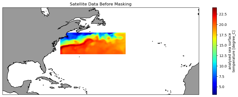

Create the region from the shape file

The plot shows the shape of the region and its placement along the US East Coast.

region = regionmask.from_geopandas(gulf_stream)
region.plot()

Mask the satellite data

# Create the mask
mask = region.mask(ds_subset.longitude, ds_subset.latitude)

# Apply mask the the satellite data
masked_ds = ds_subset.where(mask == region.numbers[0])

Visualize the masked data on a map

These data have been trimmed to contain only values within the Gulf Stream Province

plt.figure(figsize=(14, 10))

# Label axes of a Plate Carree projection with a central longitude of 180:
ax1 = plt.subplot(211, projection=ccrs.PlateCarree(central_longitude=180))

# Use the lon and lat ranges to set the extent of the map
# the 120, 260 lon range will show the whole Pacific
# the 15, 55 lat range with capture the range of the data
ax1.set_extent([260, 350, 15, 55], ccrs.PlateCarree())

# set the tick marks to be slightly inside the map extents

# add feature to the map
ax1.add_feature(cfeature.LAND, facecolor='0.6')
ax1.coastlines()

# format the lat and lon axis labels
lon_formatter = LongitudeFormatter(zero_direction_label=True)
lat_formatter = LatitudeFormatter()
ax1.xaxis.set_major_formatter(lon_formatter)
ax1.yaxis.set_major_formatter(lat_formatter)

masked_ds[0].plot.pcolormesh(ax=ax1,
                             transform=ccrs.PlateCarree(),
                             cmap='jet')

plt.title('Satellite Data After Masking for Longhurst GFST')

Text(0.5, 1.0, 'Satellite Data After Masking for Longhurst GFST')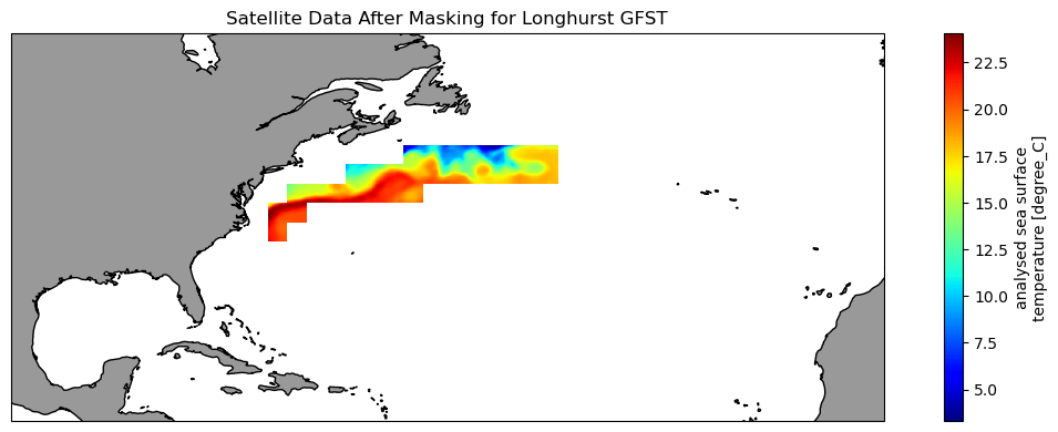

Plot the mean seasonal temperature for the province

gulf_stream_mean = masked_ds.mean(dim=['latitude', 'longitude'])

gulf_stream_mean

plt.figure(figsize=(10, 5)) 
# Plot the SeaWiFS data
plt.plot_date(gulf_stream_mean.time,
              gulf_stream_mean, 
              'o', markersize=8, 
              label='gulf stream', c='black', 
              linestyle='-', linewidth=2) 

plt.title('Gulf Stream Province Monthly Mean Temperature 2020')
plt.ylabel('SST(degrees C)') 
plt.legend()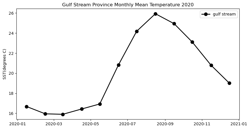

References

The several CoastWatch Node websites have data catalog containing documentation and links to all the datasets available:
* https://oceanwatch.pifsc.noaa.gov/doc.html
* https://coastwatch.pfeg.noaa.gov/data.html
* https://polarwatch.noaa.gov/catalog/

Sources for marine shape files * https://www.marineregions.org/downloads.php