Working with data that crosses the antimeridian

Background

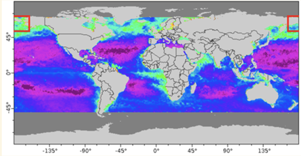
Many datasets use a system where longitude is numbered from -180 to +180 degrees east (see example below). This numbering system presents a problem for researchers working in a region that spans the antimeridian, because the parts of the data end up on the opposite ends of the map.

Figure. Global map on -180/+180 longitude showing data region crossing the antimeridian.

Objectives

This tutorial will demonstrate how to use datasets with -180 to +180 longitude values to work within regions that cross the antimeridian.

The tutorial demonstrates the following techniques

Downloading data that crosses the antimeridian from a dataset with -180 to +180 longitude values
Convert the data to a 0-360 longitude values
Reordering the longitude axis so that the longitude values are in ascending order
Visualizing data on a map

Datasets used

NOAA Chlorophyll Gap-filled, Blended NOAA-20 and S-NPP VIIRS, Science Quality, Global, 9km, 2018- recent, Daily
This NOAA dataset blends chlorophyll data from the Visible and Infrared Imager/Radiometer Suite (VIIRS) sensors aboard the Suomi-NPP and NOAA-20 spacecraft. The gaps in the data are then filled using an empirical orthogonal function (DINEOF). The dataset is available from the CoastWatch Central ERDDAP: https://coastwatch.noaa.gov/erddap/griddap/noaacwNPPN20VIIRSSCIDINEOFDaily

Import packages

import xarray as xr
import numpy as np
import matplotlib.pyplot as plt
import matplotlib as mpl

Define the area to extract

We will extract data for an area in the Bering Sea between Russia and the United States at 176°E to -152°E longitude and 50°N to 70°N latitude.

Set up variables

Date to extract
Minimum and maximum values for the longitude and latitude ranges.

my_date = '2023-08-18'
lon_min = -152.
lon_max = 176.
lat_min = 50.
lat_max = 70.

Get the SeaWiFS data

Open an xarray dataset object

#url = 'https://coastwatch.noaa.gov/erddap/griddap/noaacwNPPN20VIIRSSCIDINEOFDaily'

url = '/'.join(['https://coastwatch.noaa.gov',
                'erddap',
                'griddap',
                'noaacwNPPN20VIIRSSCIDINEOFDaily'
                ])

ds = xr.open_dataset(url)
ds

Subset the data

We will do this in two steps to make the process easier to follow. 1. Subset the data for date and latitude range 2. Subset the area around the antimeridian * Request data < the limit (-152) on the US side of the antimeridian, i.e. -180 to -152 * Request data > the limit (176) on the Russian side of the antimeridian, i.e. 176 to 180

# The lat1 and lat2 values are used in the slice function
# At first we set them as if the dataset is compliant with standards
lat1 = lat_min
lat2 = lat_max

# Then switch them if latitude values are descending
if ds.latitude[0].item() > ds.latitude[-1].item():
    lat1 = lat_max
    lat2 = lat_min

# Subset the data in two steps to make it easier to understand
# 1. Subset the date and latitude range
ds_subset = ds['chlor_a'].sel(time=my_date, 
                              method='nearest').sel(latitude=slice(lat1, lat2))

# 2. Subset the around the antimeridian
ds_subset = ds_subset.sel(longitude=(ds.longitude < lon_min) 
                          | (ds.longitude > lon_max)
                          )

ds_subset

Plot the downloaded data

# Make plot area
fig, ax = plt.subplots(figsize=(7, 5))

# Set the color palette
cmap = mpl.cm.get_cmap("jet").copy()
cmap.set_bad(color='gray')

# Show image
shw = ax.imshow(np.log10(ds_subset.squeeze()), cmap=cmap, vmin=-1, vmax=2)

bar = plt.colorbar(shw, shrink=0.65)
  
# Show plot with labels
bar.set_label('Chlorophyll (log mg m-3)')
plt.show()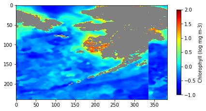

The plot of the data shows a discontinuity

The plot of subsetted data (above) shows that we downloaded the data we requested, but there is a discontinuity on the right side of the map. The data from the Russian side (west of the antimeridian) is mapped to the east of the data on the US side.

To fix the discontinuity, we need to:
* Change the longitude values on the US side of the antimeridian (-180 to -152) to values on the 0-360 longitude indexing system (180-208). * Rearrange the longitude values so that the data on the Russian side is moved to the west of the data on the US side.

Change to 0-360 longitude numbering

ds_360 = ds_subset.assign_coords(longitude=(ds_subset.longitude % 360))

print('minimum lon value =', ds_360.longitude.min().item())
print('minimum lon value =', ds_360.longitude.max().item(), end='\n\n')

print('first value in lon array =', ds_360.longitude[0].item())
print('last value in lon array =', ds_360.longitude[-1].item())

minimum lat value = 176.0416717529297
minimum lat value = 207.9583282470703

first value in lat array = 180.0416717529297
last value in lat array = 179.95834350585938

Reorder the longitude axis

The output from the cell above shows that the longitude values have been converted to 0-360. However, the lowest longitude value is not at the beginning of the array and the highest longitude value is not at the end of the array.

To rearrange the longitude values, use the roll function of xarray. The roll function will push values along an axis by the number of steps you enter. The values that are “pushed off” of the end of the array will be put at the beginning of the array.

First we need to find the position where the longitude discontinuity happens, i.e. where the most easterly longitude (208.0) abruptly meets the most easterly longitude value (176.0)
Next, use the discontinuity position to determine how many positions to roll the longitude array to the right. Apply the number to the roll function.

# This code finds the index where the absolute value between each longitude value 
# and the largest longitude value is maximal
discont_index = max(range(len(ds_360.longitude)), 
                    key=lambda i: abs(ds_360.longitude[i] -
                                      ds_360.longitude.max())
                    )
print('the index marking the discontinuity is:', discont_index, end='\n\n')

# Substract the discontinuity position from the length of the array 
# to obtain the number of positions to roll the longitude axis
postions_to_roll = len(ds_360.longitude) - discont_index

# Roll the dataset
ds_rolled = ds_360.roll(longitude=postions_to_roll, roll_coords=True)

print('minimum lon value =', ds_rolled.longitude.min().item())
print('minimum lon value =', ds_rolled.longitude.max().item(), end='\n\n')

print('first value in lon array =', ds_rolled.longitude[0].item())
print('last value in lon array =', ds_rolled.longitude[-1].item())

the index marking the discontinuity is: 336

minimum lon value = 176.0416717529297
minimum lon value = 207.9583282470703

first value in lon array = 176.0416717529297
last value in lon array = 207.9583282470703

The output from the cell above shows that the longitude values have been converted to 0-360, and that the lowest longitude value is at the beginning of the array and the highest longitude value is at the end of the array.

Plot the data

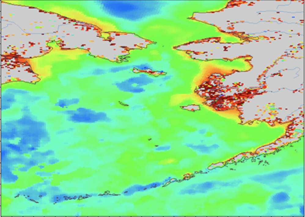
The discontinuity has been corrected!

# Make plot area
fig, ax = plt.subplots(figsize=(7, 5))

# Set the color palette
cmap = mpl.cm.get_cmap("jet").copy()
cmap.set_bad(color='gray')

# show image
shw = ax.imshow(np.log10(ds_rolled.squeeze()), 
                cmap=cmap,
                vmin=-1, 
                vmax=2)

bar = plt.colorbar(shw, shrink=0.65)
  
# show plot with labels
bar.set_label('Chlorophyll (log mg m-3)')
plt.show()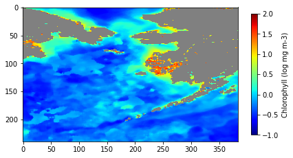

Save the corrected dataset as a netCDF file

ds_rolled.to_netcdf('data_corrected_0_to_360.nc')