import cartopy.crs as ccrs
import urllib.request
import xarray as xr
import numpy as np
from pyproj import CRS
from pyproj import Transformer
from matplotlib import pyplot as plt
import cmoceanTransforming satellite data from one map projection to another
History | Create July 2023 | Updated August 2023
Background
Map projections try to portray the earth’s spherical surface on a flat surface. A coordinate reference system (CRS) defines how the two-dimensional, projected map relates to real places on the earth. Which map projection and CRS to use depends on the region in which you are working and the analysis you will do.
NOAA PolarWatch distributes gridded and tabular oceanographic data for polar regions.
Most of the satellite data in the PolarWatch data catalog use a projection based on a Geographic Coordinate Reference System, where the X and Y coordinates are longitude and latitude, respectively. Geographical coordinates work well in many parts of the globe, but within polar regions, features tend to be very distorted. A Polar Stereographic projection often is a better choice for polar regions. For example, the NSIDC’s Polar Stereographic Projections, which were developed to optimize mapping of sea ice, have only a 6% distortion of the grid at the poles and no distortion at 70º, a latitude close to where the marginal ice zones occur. The NOAA NSIDC Sea Ice Concentration Climate Data Record dataset, for example, is in a polar stereographic projection.
When working with satellite datasets with a mix of map projections, it is often necessary to transform all the data to a common projection.
Objective
In this tutorial, we will learn to transform dataset coordinates from one projection to another.
This tutorial demonstrates the following techniques
- Downloading and saving a netCDF file from PolarWatch ERDDAP data server
- Accessing satellite data and metadata in polar stereographic projection
- Transforming coordinates using EPSG codes
- Mapping data using the transformed coordinates
Datasets used
Sea Ice Concentration, NOAA/NSIDC Climate Data Record V4, Southern Hemisphere, Science Quality, 1978-2022, Monthly
The sea ice concentration (SIC) dataset used in this exercise is produced by NOAA NSIDC from passive microwave sensors as part of the Climate Data Record. It is a science quality dataset of monthly averages that extends from 1978-2022. SIC is reported as the fraction (0 to 1) of each grid cell that is covered by ice. The data are mapped in the Southern Polar Stereographic projection (EPSG:3031). The resolution is 25km, meaning each pixel in this data set represents a value that covers a 25km by 25km area. The dataset can be downloaded directly from the PolarWatch ERDDAP at the following link: https://polarwatch.noaa.gov/erddap/griddap/nsidcG02202v4shmday
Import packages
## Get data from ERDDAP
# request data from polarwatch.noaa.gov erddap and save it to sic.nc file

url = ''.join(["https://polarwatch.noaa.gov/erddap/griddap/",
               "nsidcG02202v4shmday.nc?cdr_seaice_conc_monthly",
               "[(2022-12-01T00:00:00Z):1:(2022-12-01T00:00:00Z)]",
               "[(4350000.0):1:(-3950000.0)][(-3950000.0):1:(3950000.0)]"
               ])

urllib.request.urlretrieve(url, "sic.nc")
# open and assign data from the file to a variable ds using xarray
ds = xr.open_dataset("sic.nc")
# view metadata
dsInspect CRS definitions and the transformation function
When transforming from one CRS to another, it is important to inspect CRS definitions and the transformation function for proper transformation. We will transform from CRS EPSG: 3031 (NSIDC Polar Stereographic South) to EPSG: 4326 (geographic coordinate system) .
There are several ways to specify CRS as shown below. For this exercise, we will use EPSG code.
1. crs = CRS.from_epsg(4326)
2. crs = CRS.from_string("EPSG:4326")
3. crs = CRS.from_proj4("+proj=latlon")
For this exercise, we will use method 1, the EPSG code.
Get the projection information from the EPSG code
Geographic
crs_4326 = CRS.from_epsg(4326)
crs_4326
NSIDC Polar Stereographic South
crs_3031 = CRS.from_epsg(3031)
crs_3031
Inspect CRS definitions
crs_4326 * order of axis: latitude first, and longitude in degree * bounds (-180, -90, 180, 90) global coverage
crs_3031 * order of axis: X then Y in meter * bounds (-180, -90, 180, -60)
based on the crs definitions * transformation input should be in the order of latitude and longitude * transformation input/output should be within the bounds
NOTE: if you prefer to use lon and lat (or x, y) axis order, you can set transformer parameter always_xy to True
Transformer.from_crs(crs_3031, crs_4326, always_xy=True)
Transform the data
# transformer converts lon and lat values to x, y
transformer = Transformer.from_crs(crs_3031, crs_4326)

# create a rectangular grid
x, y = np.meshgrid(ds.xgrid, ds.ygrid)

# pass x and y grid values to transform
lat, lon = transformer.transform(x,y)
Add latitude and longitude values to the dataset
For adding the new coordinates to the dataset, create a tuple with its dimension and values then add to the dataset.
- create a tuple
(dimension, value) - add to the dataset (ds)
ds.coord['name']=(dimension, value)
ds.coords['lat'] = (ds.cdr_seaice_conc_monthly[0][:].dims, lat)
ds.coords['lon'] = (ds.cdr_seaice_conc_monthly[0][:].dims, lon)

ds['cdr_seaice_conc_monthly'] = (ds['cdr_seaice_conc_monthly']
                                 .where(ds['cdr_seaice_conc_monthly'] <= 1,
                                        np.nan)
                                 )
Plot data with new coordinates on a global map
Because the data were in the polar stereographic projection, mapping the data onto a different projection (global map projection) below, doesn’t make the data fit well on the map.
# set the map size
plt.figure(figsize=(13,5))

# set map projection (PlateCarree(): global map projection)
ax = plt.axes(projection=ccrs.PlateCarree())

# plot data with new coordinates
ds.cdr_seaice_conc_monthly[0][:].plot.pcolormesh('lon',
                                                 'lat',
                                                 ax=ax,
                                                 transform=ccrs.PlateCarree(),
                                                 cmap=cmocean.cm.ice,
                                                 add_colorbar=False)
# add coastlines to the map
ax.coastlines()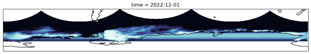
Plot data with new coordinates on a polar stereographic projection map
# Set map projection
# SouthPolarStereo(): southern polar stereographic projection)
ax = plt.axes(projection=ccrs.SouthPolarStereo())

ds.cdr_seaice_conc_monthly[0][:].plot.pcolormesh('lon',
                                                 'lat',
                                                 ax=ax,
                                                 cmap=cmocean.cm.ice,
                                                 transform=ccrs.PlateCarree())

ax.coastlines()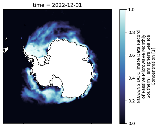
References
Useful links