Calculate sea ice extent
notebook filename | sea_ice_extent.Rmd
Background
Sea ice cover measurements are key to polar ecological and climatological research. This measurement has gained attention because of the recent decrease in the Arctic sea ice cover. Satellite observations are essential for tracking sea ice cover, providing continuous global coverage extending back to 1978. Typically, sea ice cover is reported as sea ice concentration, which is the percent areal coverage of ice within a grid cell. Depending on the application, additional parameters of interest can be calculated from sea ice cover:
- Sea ice area - the cumulative coverage of all gridded sections (area), including each grid that contains a minimum ice concentration of 15%.
- Sea ice extent - the cumulative coverage of all griddedthe sum of the areas of all grid cells with at least 15% ice concentration
Objective
This tutorial will demonstrate how to calculate the sea ice area and extent using sea ice concentration and grid cell area data. Please visit the NSIDC website for more detailed descriptions of the calculations.
The tutorial demonstrates the following techniques
- Downloading and saving a netcdf file from the PolarWatch ERDDAP data server
- Accessing satellite data and metadata in polar stereographic projection
- Downloading and adding grid cell area data to the satellite data
- Visualizing data on a map
- Computing sea ice area and extent using sea ice concentration data
- Plotting a time series of sea ice area and extent
Datasets used
Sea Ice Concentration, NOAA/NSIDC Climate Data Record V4, Northern Hemisphere.
The Sea ice concentration (SIC) dataset used in this exercise is produced by NOAA NSIDC from passive microwave sensors as part of the Climate Data Record. It is a science quality dataset of monthly averages that extends from 1978-2022. Near-Real-Time data are also available at PolarWatch. (SIC is reported as the fraction (0 to 1) of each grid cell that is covered by ice. The data are mapped in the Northern Polar Stereographic projection (EPSG:3413). The resolution is 25km, meaning each grid cell in this data set represents a value that covers a 25km by 25km area. The dataset is available on the PolarWatch data portal and can be downloaded directly from the PolarWatch ERDDAP at the following link: https://polarwatch.noaa.gov/erddap/griddap/nsidcG02202v4nhmday.graph
Polar Stereographic Grid Cell Area Values of 25km grid, Polar Stereographic (North), NSIDC Ancillary Data.
This dataset includes the area (in m2) of each grid cell in the 25km resolution Northern Polar Stereographic projection. This dataset is available on the PolarWatch ERDDAP
# Function to check if pkgs are installed, install missing pkgs, and load
pkgTest <- function(x)
{
  if (!require(x,character.only = TRUE))
  {
    install.packages(x,dep=TRUE,repos='http://cran.us.r-project.org')
    if(!require(x,character.only = TRUE)) stop(x, " :Package not found")
  }
}

list.of.packages <- c( "ggplot2" ,"ncdf4",  "RColorBrewer", "scales")

# create list of installed packages
pkges = installed.packages()[,"Package"]
for (pk in list.of.packages) {
  pkgTest(pk)
}

# Set up download method as libcurl, this is only needed for Windows machines
options(download.file.method="libcurl", url.method="libcurl")
Get the sea ice data from ERDDAP
Here we download the average monthly sea ice concentration for the Arctic for 2021 (January to December). We are using the NSIDC Sea Ice Concentration Climate Data Record (NSIDC ID: G002202).
The ERDDAP data request URL for this data subset is presented below.
https://polarwatch.noaa.gov/erddap/griddap/nsidcG02202v4nhmday.nc?cdr_seaice_conc_monthly[(2021-01-01T00:00:00Z):1:(2021-12-01T00:00:00Z)][(5837500.0):1:(-5337500.0)][(-3850000.0):1:(3750000.0)]The following table shows the component parts of the ERDDAP data request URL.
| Name | Value | Description |
|---|---|---|
| base_url | https://polarwatch.noaa.gov/erddap/griddap | ERDDAP URL for gridded datasets |
| datasetID | nsidcG02202v4nhmday | Unique ID of the dataset from PolarWatch ERDDAP |
| file_type | .nc | NetCDF (there are many other available file formats) |
| query_start | ? | Details of the query follow the ? |
| variable_name | cdr_seaice_conc_monthly | Variables from the dataset |
| date_range | [(2021-01-01T00:00:00Z):1:(2021-12-01T00:00:00Z)] | Temporal |
| spatial_range | [(5837500.0):1:(-5337500.0)][(-3850000.0):1:(3750000.0)] | Spatial coverage |
` Note The metadata states that the _FillValue for this dataset is set to -999, however when the _FillValue attribute is found, the ncdf4 package maps all the missing values (_FillValue) to NA’s.
# Set data request URL for PolarWatch ERDDAP data server
data_url <- "https://polarwatch.noaa.gov/erddap/griddap/nsidcG02202v4nhmday.nc?cdr_seaice_conc_monthly[(2021-01-01T00:00:00Z):1:(2021-12-01T00:00:00Z)][(5837500.0):1:(-5337500.0)][(-3850000.0):1:(3750000.0)]"


# Send data request and download file to the file name
f <- 'sic.nc'
download.file(data_url, destfile=f, mode="wb")
# Open netcdf file
nc=nc_open('sic.nc')
# Examine file metadata
#print(nc)
# Examine names of variables
names(nc$var)
# Get first variable metadata
var1 <- nc$var[[1]]
# Examine variable metadata
#print(var1)
# Get variable values
sic <- ncvar_get(nc,var1$name)
# Examine dimension of variables
dim(sic)
# Based on metadata, set xgrid, ygrid
xgrid <- var1$dim[[1]]$vals
ygrid <- var1$dim[[2]]$vals
# convert time variable to date format
dates <- as.POSIXlt(var1$dim[[3]]$vals,origin='1970-01-01',tz='GMT')# Close and remove the netCDF file and clear memories
nc_close(nc)
file.remove('sic.nc')## [1] TRUEPlot Sea Ice Concentration Data
To plot sea ice concentration data that are in xgrid and ygrid dimensions, we will create a data frame with coordinates (xgrid, ygrid) and associated sea ice concentration values.
# Create a data frame with all combinations of xgrid and ygrid
sicd <- expand.grid(xgrid=xgrid, ygrid=ygrid)

# Add sic data array to the data frame
sicd$sic <- array(sic, dim(xgrid)*dim(ygrid))

# exclude the _FillValue listed in the metadata (2.53999) which corresponds to various pixels with no data (land, coast, missing data, etc...)
sicd$sic[sicd$sic > 2] <- NA

# Map sea ice concentration
ggplot(data = sicd, aes(x = xgrid, y = ygrid, fill=sic) ) +
       geom_tile() +
       coord_fixed(ratio = 1) +
       scale_y_continuous() +
       scale_x_continuous() +
       scale_fill_gradientn(colours=rev(brewer.pal(n = 3, name = "Blues")),na.value="tan") +
      ggtitle("Sea Ice Concentration on Polar Steregraphic projection")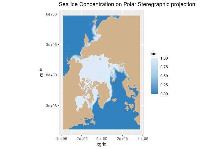
Download grid cell area values
While the resolution of this data set is 25km, the actual area of each grid cell depends on the grid projection. We will download the grid cell area values from the PolarWatch ERDDAP.
cell_url <- "https://polarwatch.noaa.gov/erddap/griddap/pstere_gridcell_N25k.nc?cell_area%5B(5837500.0):1:(-5337500.0)%5D%5B(-3837500.0):1:(3737500.0)%5D"
f <- 'gridcell.nc'
download.file(cell_url, destfile=f, mode="wb")
Examine grid cell dataset metadata and extract values
Just like for the sea ice concentration dataset, we will examine the metadata and extract the variables of grid cell areas along with x and y grids.
# Open netcdf file
nc1=nc_open('gridcell.nc')

# Examine names of variables
names(nc1$var)

# Get first variable metadata
area_var <- nc1$var[[1]]

# Examine area_var
names(area_var)

# Get variable values
cellarea =ncvar_get(nc1,area_var$name)

# Examine dimension of variable values
dim(cellarea)

# Based on metadata, set xgrid, ygrid, time
x_area <- area_var$dim[[1]]$vals
y_area <- area_var$dim[[2]]$vals

# Close and remove the netCDF file and clear memories
nc_close(nc1)
file.remove('gridcell.nc')
Match cell area grids with SIC grids
Now we have two data sets: sea ice concentration and grid cell areas for each grid of northern polar stereographic projection. While the spatial coverage of both data sets is identical, we will ensure the x and y coordinates of both data sets are correctly aligned.
# Get indices in areas where x and y grids equal those of sic
x_indices <- match(xgrid, x_area)
y_indices <- match(ygrid, y_area)

# Extract grid area
grid.match <- cellarea[x_indices, y_indices]
Clean sea ice concentration data for sea ice area calculation
We need to clean the data before computing the sea ice area and extent.
- The dataset includes flag values indicating non-sea ice area such as land, lakes, etc.
- task: remove flag values (2 and higher) by setting the flag values as Nan.
- For this example of the sea ice area and extent calculations, a value of 0.15 of sea ice concentration value will be used as a threshold.
- task: set sic value to 0 if the value is less than 0.15
For more detailed information about the flag values, go to the user guide. For the calculation of sea ice area and extent with a threshold, go to the NSIDC article.
# Set sic values less than 0.15 to (applying 0.15 threshold)
sic[sic < 0.15] <- 0

# Set 0 for all flag values (>2)
sic[sic > 1] <- 0

# Set NA to 0
sic[is.na(sic)] <- 0

# Sic for extent calc
sic_ext <- sic
sic_ext[sic_ext >= 0.15] <- 1


# Perform element-wise multiplication for the first time step
area_total <- sic[,,1] * grid.match
ext_total <- sic_ext[,,1] * grid.match

# Sum area and extent over all grid cells and convert from m^2 to km^2
area <- sum(area_total) / 1000000
extent <- sum(ext_total) / 1000000

print(paste("Sea Ice Area (km^2): ", floor(area)))
## [1] "Sea Ice Area (km^2): 12564015"print(paste("Sea Ice Extent (km^2): ", floor(extent)))## [1] "Sea Ice Extent (km^2): 13905993"Generate the sea ice area and extent time series
# Replicate grid areas for all timestep
rep_grid_areas <- array(rep(grid.match, each=dim(sic)[3]), dim=dim(sic))

# Perform element-wise multiplication
area_total12 <- sic * rep_grid_areas
ext_total12 <- sic_ext * rep_grid_areas

area12 <- apply(area_total12, c(3), sum)
ext12 <- apply(ext_total12, c(3), sum)
Plot the sea ice area and extent time series
upper = max(max(ext12), max(area12))
lower = min(min(ext12), min(area12))
plot(dates,ext12,type='o',pch=20,xlab='Date',ylab='Area (km^2)', col="orange" , ylim=c(lower, upper),  main="2021 Monthly Sea ice area and sea ice extent")
lines(dates, area12, type='o', pch=20, col="blue")
legend("topright", legend=c("Sea ice Area", "Sea ice Extent"),
       col=c("blue", "orange"), lty=1:1, cex=0.8)
box()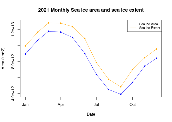
References
- NSIDC Data Product Description
- NSIDC Data Product User Guide (pdf)
- PolarWatch Data Catalog
- What’s the difference between Sea ice area and extent?
- NSIDC Arctic Sea Ice News & Analysis
- Climate.gov Understanding Climate: sea ice extent
- Several CoastWatch Node websites have data catalogs containing documentation and links to all the datasets available: